Как пишется индукция в физике - Граматика и образование на Pisanino.ru

Индукция электрическая и магнитная, физические величины, характеризующие (наряду с напряжённостями электрического и магнитного полей) электромагнитное поле. В вакууме эти характеристики совпадают с соответствующими напряжённостями, если пользоваться СГС системой единиц (Гаусса); в Международной системе единиц (СИ) они различаются постоянными множителями.

Вектор электрической индукции D (называемый также электрическим смещением) является суммой двух векторов различной природы: напряжённости электрического поля Е ‒ главной характеристики этого поля ‒ и поляризации Р, которая определяет электрическое состояние вещества в этом поле. В системе Гаусса:

D = E + 4pP

(1)

(4p ‒ постоянный коэффициент); в системе СИ

D = e0E + P,

(1¢)

где e0 ‒ размерная константа, называемая электрической постоянной или диэлектрической проницаемостью вакуума. Вектор поляризации Р представляет собой электрический дипольный момент единицы объёма вещества в поле Е, т. е. сумму электрических дипольных моментов pi, отдельных молекул внутри малого объёма DV, деленную на величину этого объёма:

В изотропном веществе, не обладающем сегнетоэлектрическими свойствами (см. Сегнетоэлектричество), при слабых полях вектор поляризации прямо пропорционален напряжённости поля. В системе Гаусса

P = cеЕ,

(3)

где ce ‒ безразмерная величина, называемая коэффициентом поляризации или диэлектрической восприимчивостью. Именно она характеризует электрические свойства вещества. Для сегнетоэлектриков ce зависит от Е, так что связь Р и Е становится нелинейной.

Подставляя выражение (3) в (1), получим:

D = (1 + 4pcе)Е = eЕ.

(4) Величина

e = 1 + 4pce,

(5)

также характеризующая электрические свойства вещества, называется диэлектрической проницаемостью. В системе СИ

Р = ce e0E

(3¢)

и, соответственно,

D = e0eЕ,

(4▓)

e = 1 + ce.

(5▓)

Смысл введения вектора электрической И. состоит в том, что поток вектора D через любую замкнутую поверхность определяется только свободными зарядами, а не всеми зарядами внутри объёма, ограниченного данной поверхностью, подобно потоку вектора Е. Это позволяет не рассматривать связанные (поляризационные) заряды и упрощает решение многих задач.

Вектор магнитной индукции В ‒ основная характеристика магнитного поля, представляющая собой среднее значение суммарной напряжённости микроскопических магнитных полей, созданных отдельными электронами и др. элементарными частицами. Вектор же напряжённости магнитного поля Н является разностью двух векторов различной природы: вектора В и вектора намагниченности I. В системе Гаусса

Н = В ‒ 4pI,

Или

(6)

В = Н + 4pI.

Намагниченность представляет собой магнитный момент единицы объёма и характеризует магнитное состояние вещества. В изотропной среде при слабых полях намагниченность прямо пропорциональна Н:

I = cm H,

(7)

где cm ‒ магнитная восприимчивость, характеризующая магнитные свойства вещества. Для ферромагнетиков cm зависит от Н. Подставляя (7) в (6), получим связь между В и Н :

В = (1 + 4pcm)H = mН

(8)

Величина

m = 1 + 4pcm,

(9)

также характеризующая магнитные свойства вещества, называется магнитной проницаемостью.

В системе СИ эти формулы записываются следующим образом:

В = m0H + I,

(6′)

I = m0cm H,

(7′)

В = m0mН,

(8′)

m = 1 + cm

(9′)

Константа m0 называется магнитной постоянной или магнитной проницаемостью вакуума. Вектор Н вводится в теорию электромагнитного поля в связи с тем, что циркуляция вектора Н вдоль замкнутого контура, в отличие от циркуляции вектора В, определяется движением только свободных зарядов.

Лит.: Калашников С. Г., Электричество, М., 1970 (Общий курс физики, т. 2), гл. 5 и 11; Фриш С. Э. и Тиморева А. В., Курс общей физики, т. 2, М., 1953, гл. 15, 18.

Г. Я. Мякишев.

Большая советская энциклопедия. — М.: Советская энциклопедия.
1969—1978.

Источник

Магнитное поле относится к силовым физическим величинам – воздействует на проводник, пропускающий электрический ток. Зависит от активной длины проводника, силы Ампера и протекающего тока. Ознакомимся подробнее с понятием магнитная индукция, формулой для её вычисления, причинами появления, практическим использованием.

Теория

Магнитное поле относится к силовым, значит, его характеризуют индукцией. Последняя обнаруживается двумя путями:

по наличию силы Ампера, оказывающей воздействие на прямой проводник, пропускающий электрический ток;
пиковым вращающим моментом, действующим на закрытый контур с магнитным моментом.

Исследуя магнитные поля посредством проводящего электричество проводника, модуль их индукции вычисляется как отношение пикового значения силы Ампера FA, оказывающей воздействие на проводник к произведению силы проходящего по нему тока, умноженную на активную длину проводящего ток провода. Магнитное поле относится к однородным, если в его точках вектор B одинаков по модулю и направлению.

Направление индукции определяется по следующему алгоритму:

Прямолинейный проводник ориентируется в поле так, чтобы действовала как можно большая сила FA.
Левая рука с раскрытой ладонью помещается у проводника.
Четыре пальца указывают на направление протекания тока.
Большой палец отгибается на 90°, указывает направление F_A.
Вектор индукции направлен в раскрытую ладонь под углом 90°.

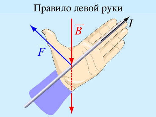
Алгоритм называется правилом левой руки.

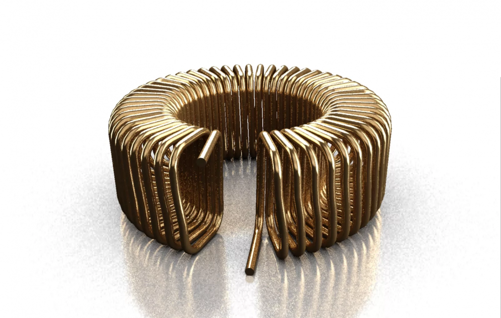
Вектор индукции для соленоида входит в катушку со стороны, где ток двигается по ходу часовой стрелки.

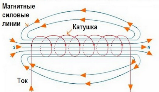
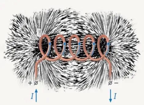
Силовые линии обнаруживаются и при помощи металлических опилок.

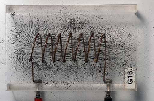
Изменяя параметры поля и соленоида, формируют интересные узоры.

Магнитная индукция: формула, единица измерения

В физике индукция магнитного поля обозначается буквой B. Вычисляется по формуле:

B= F / Il, здесь:

F – максимальная сила Ампера;
I – значение тока;
l – длина проводника.

Единица измерения B: Н / (А*м) = 1 Тл – Тесла. Названа в честь югославского физика и изобретателя Никола Тесла.

Исследуя магнитную составляющую проводника при помощи замкнутого контура, направление вектора B принимают за направление, расположенное под 90° к плоскости, где установлен вращающийся контур.

По модулю B также равняется отношению пикового момента сил M, оказывающего воздействие на контур с током, к величине тока, протекающего по рамке, и её площади:

B = M / IS.

Единица измерения совпадает с описанной ранее: Н*м /А*м²= Н / А* м = 1 Тл.

Задача

Вычислить индукцию куска провода длиной 10 см, расположенного в магнитном поле 50 мН, если по нему протекает ток 5 А.

B = F / Il. Всё известно, подставляем значения в формулу.

B = 0,05 / (5*0,1) = 0,2 Тл.

Ответ: индукция равняется 0,02 Тл.

Источник

Формула индукции магнитного поля

Направлением вектора магнитной индукции считают направление на север магнитной стрелки, которая может свободно вращаться в магнитном поле. Такое же направление имеет положительная нормаль к замкнутому контуру, по которому течет ток. Положительная нормаль имеет направление, совпадающее с направлением перемещения правого винта (буравчика), если его вращают по направлению тока в контуре.

Модуль вектора магнитной индукции можно установить, используя силу, которая действует на проводники с током, помещенные в магнитное поле (силу Ампера). Тогда модуль вектора равен частному от деления максимальной силы ( $F_{max}$ ), с которой магнитное поле оказывает воздействие на отрезок проводника с током (I) к произведению силы тока на длину проводника ():

$[B=frac{F_{max}}{IDelta l} qquad(1)]$

Рассматривая силу Лоренца, которая действует на заряженную частицу, движущуюся в магнитном поле, получают формулу для магнитной индукции в виде:

$[B=frac{F_L}{qvsin alpha } } qquad(2)]$

где – модуль силы Лоренца; q – заряд частицы, движущейся со скоростью v в магнитном поле; – это угол между векторами и . Направления ${overline{F}}_L$ , векторов и связаны между собой правилом левой руки.

Формулой, которая определяет величину вектора магнитной индукции в данной точке магнитного поля, считают так же следующее выражение:

$[B=frac{M_{max}}{p_m} qquad(3)]$

где $M_{max}$ – максимальный вращающий момент, действующий на рамку, которая обладает магнитным моментом , равным единице, если нормаль к рамке перпендикулярна направлению поля. Вращающий момент (M), действующий на контур с током I в однородном магнитном поле можно вычислить как:

где S – площадь, которую обтекает ток I. Следует помнить, что максимальный вращающий момент получается тогда, когда плоскость контура параллельна линиям магнитной индукции поля ().

Принцип суперпозиции магнитных полей

Если магнитное поле получается в результат наложения нескольких магнитных полей то, магнитная индукция поля (), может быть найдена как векторная сумма магнитных индукций отдельных полей ( ${overline{B}}_i$ ):

$[overline{B}=sum^N_{i=1}{{overline{B}}_i} qquad(5)]$

Закон Био-Савара-Лапласа, как формула для вычисления величины индукции магнитного поля

Закон Био-Савара – Лапласа является одним из распространенных законов, который позволяет вычислить вектор магнитной индукции () в любой точке магнитного поля, создаваемого в вакууме элементарным проводником с током:

$[doverline{B}=frac{{mu }_0}{4pi }frac{I}{r^3}left[doverline{l}overline{r}right] qquad(6)]$

где I – сила тока; – вектор элементарный проводник по модулю он равен длине проводника, при этом его направление совпадает с направлением течения тока; – радиус-вектор, который проводят от элементарного проводника к точке, в которой находят поле; ${mu }_0=4pi cdot {10}^{-7}frac{Гн}{м}$ – магнитная постоянная. Вектор является перпендикулярным к плоскости, в которой расположены и , конкретное направление вектора магнитной индукции определяют при помощи правила буравчика (правого винта).

Для однородного и изотропного магнетика, заполняющего пространство, вектор магнитной индукции в вакууме( ${overline{B}}_0)$ и в веществе (), при одинаковых условиях, связывает формула:

$[overline{B}=mu {overline{B}}_0 qquad(7)]$

где – относительная магнитная проницаемость вещества.

Частные случаи формул для вычисления модуля вектора магнитной индукции

Формула для вычисления модуля вектора индукции в центре кругового витка с током (I):

$[B=frac{{mu }_0mu }{2}frac{I}{R} qquad(8)]$

где R – радиус витка.

Модуль вектора магнитной индукции поля, которое создает бесконечно длинный прямой проводник с током:

$[B=frac{{mu }_0mu }{2pi }frac{I}{r} qquad(9)]$

где r – расстояние от оси проводника до точки, в которой рассматривается поле.

В средней части соленоида магнитная индукция поля вычисляется при помощи формулы:

$[B={mu }_0mu nI left(10right)]$

где n – количество витков соленоида на единицу длины; I – сила тока в витке.

Примеры решения задач по теме «Индукция магнитного поля»

Источник

Магнитный поток

Прежде, чем разобраться с тем, что такое электромагнитная индукция, нужно определить такую сущность, как магнитный поток.

Представьте, что вы взяли обруч в руки и вышли на улицу в ливень. Чем сильнее ливень, тем больше через этот обруч пройдет воды — поток воды больше.

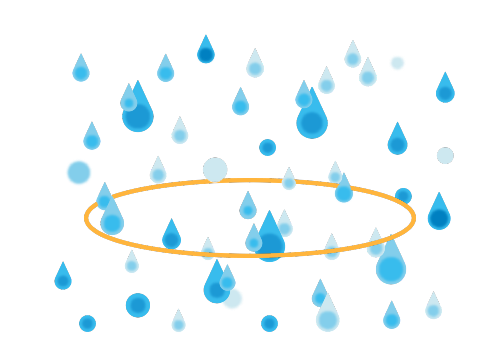
Если обруч расположен горизонтально, то через него пройдет много воды. А если начать его поворачивать — уже меньше, потому что он расположен не под прямым углом к вертикали.

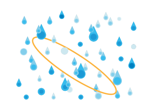
Теперь давайте поставим обруч вертикально — ни одной капли не пройдет сквозь него (если ветер не подует, конечно).

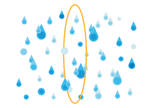
Магнитный поток по сути своей — это тот же самый поток воды через обруч, только считаем мы величину прошедшего через площадь магнитного поля, а не дождя.

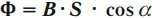
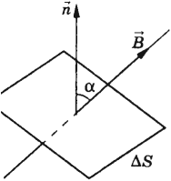
Магнитным потоком через площадь S контура называют скалярную физическую величину, равную произведению модуля вектора магнитной индукции B, площади поверхности S, пронизываемой данным потоком, и косинуса угла α между направлением вектора магнитной индукции и вектора нормали (перпендикуляра к плоскости данной поверхности):

Магнитный поток

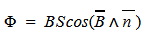
Ф — магнитный поток [Вб]

B — магнитная индукция [Тл]

S — площадь пронизываемой поверхности [м^2]

n — вектор нормали (перпендикуляр к поверхности) [-]

Магнитный поток можно наглядно представить как величину, пропорциональную числу магнитных линий, проходящих через данную площадь.

В зависимости от угла α магнитный поток может быть положительным (α < 90°) или отрицательным (α > 90°). Если α = 90°, то магнитный поток равен 0. Это зависит от величины косинуса угла.

Изменить магнитный поток можно меняя площадь контура, модуль индукции поля или расположение контура в магнитном поле (поворачивая его).

В случае неоднородного магнитного поля и неплоского контура, магнитный поток находят как сумму магнитных потоков, пронизывающих площадь каждого из участков, на которые можно разбить данную поверхность.

Практикующий детский психолог Екатерина Мурашова

Бесплатный курс для современных мам и пап от Екатерины Мурашовой. Запишитесь и участвуйте в розыгрыше 8 уроков

Электромагнитная индукция

Электромагнитная индукция — явление возникновения тока в замкнутом проводящем контуре при изменении магнитного потока, пронизывающего его.

Явление электромагнитной индукции было открыто М. Фарадеем.

Майкл Фарадей провел ряд опытов, которые помогли открыть явление электромагнитной индукции.

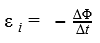
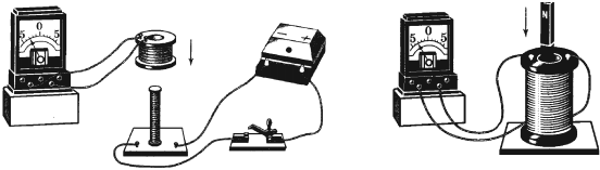
Опыт раз. На одну непроводящую основу намотали две катушки: витки первой катушки были расположены между витками второй. Витки одной катушки были замкнуты на гальванометр, а второй — подключены к источнику тока.

При замыкании ключа и протекании тока по второй катушке в первой возникал импульс тока. При размыкании ключа также наблюдался импульс тока, но ток через гальванометр тек в противоположном направлении.

Опыт два. Первую катушку подключили к источнику тока, а вторую — к гальванометру. При этом вторая катушка перемещалась относительно первой. При приближении или удалении катушки фиксировался ток.

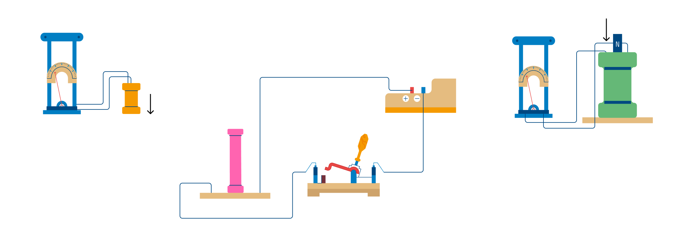
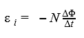
Опыт три. Катушка замкнута на гальванометр, а магнит движется вдвигается (выдвигается) относительно катушки

Вот, что показали эти опыты:

Индукционный ток возникает только при изменении линий магнитной индукции.

Направление тока будет различно при увеличении числа линий и при их уменьшении.

Сила индукционного тока зависит от скорости изменения магнитного потока. Может изменяться само поле, или контур может перемещаться в неоднородном магнитном поле.

Почему возникает индукционный ток?

Значит, при изменении числа магнитных линий через поверхность, ограниченную контуром, в нем появляется ЭДС, которую называют ЭДС индукции.

Онлайн-курсы физики в Skysmart не менее увлекательны, чем наши статьи!

Закон электромагнитной индукции

Закон электромагнитной индукции (закон Фарадея) звучит так:

ЭДС индукции в замкнутом контуре равна и противоположна по знаку скорости изменения магнитного потока через поверхность, ограниченную контуром.

Математически его можно описать формулой:

Закон Фарадея

Ɛi — ЭДС индукции [В]

ΔФ/Δt — скорость изменения магнитного потока [Вб/с]

Знак «–» в формуле позволяет учесть направление индукционного тока. Индукционный ток в замкнутом контуре всегда направлен так, чтобы магнитный поток поля, созданного этим током сквозь поверхность, ограниченную контуром, уменьшал бы те изменения поля, которые вызвали появление индукционного тока.

Если контур состоит из N витков (то есть он — катушка), то ЭДС индукции будет вычисляться следующим образом.

Закон Фарадея для контура из N витков

Ɛi — ЭДС индукции [В]

ΔФ/Δt — скорость изменения магнитного потока [Вб/с]

N — количество витков [-]

Сила индукционного тока в замкнутом проводящем контуре с сопротивлением R:

Закон Ома для проводящего контура

Ɛi — ЭДС индукции [В]

I — сила индукционного тока [А]

R — сопротивление контура [Ом]

Если проводник длиной l будет двигаться со скоростью v в постоянном однородном магнитном поле с индукцией B ЭДС электромагнитной индукции равна:

ЭДС индукции для движущегося проводника

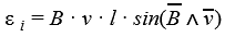
Ɛi — ЭДС индукции [В]

B — магнитная индукция [Тл]

v — скорость проводника [м/с]

l — длина проводника [м]

Возникновение ЭДС индукции в движущемся в магнитном поле проводнике объясняется действием силы Лоренца на свободные заряды в движущихся проводниках. Сила Лоренца играет в этом случае роль сторонней силы.

Движущийся в магнитном поле проводник, по которому протекает индукционный ток, испытывает магнитное торможение. Полная работа силы Лоренца равна нулю.

Количество теплоты в контуре выделяется либо за счет работы внешней силы, которая поддерживает скорость проводника неизменной, либо за счет уменьшения кинетической энергии проводника.

Изменение магнитного потока, пронизывающего замкнутый контур, может происходить по двум причинам:

вследствие перемещения контура или его частей в постоянном во времени магнитном поле. Это случай, когда проводники, а вместе с ними и свободные носители заряда, движутся в магнитном поле
вследствие изменения во времени магнитного поля при неподвижном контуре. В этом случае возникновение ЭДС индукции уже нельзя объяснить действием силы Лоренца. Явление электромагнитной индукции в неподвижных проводниках, возникающее при изменении окружающего магнитного поля, также описывается формулой Фарадея

Таким образом, явления индукции в движущихся и неподвижных проводниках протекают одинаково, но физическая причина возникновения индукционного тока оказывается в этих двух случаях различной:

в случае движущихся проводников ЭДС индукции обусловлена силой Лоренца
в случае неподвижных проводников ЭДС индукции является следствием действия на свободные заряды вихревого электрического поля, возникающего при изменении магнитного поля.

Правило Ленца

Чтобы определить направление индукционного тока, нужно воспользоваться правилом Ленца.

Академически это правило звучит следующим образом: индукционный ток, возбуждаемый в замкнутом контуре при изменении магнитного потока, всегда направлен так, что создаваемое им магнитное поле препятствует изменению магнитного потока, вызывающего индукционный ток.

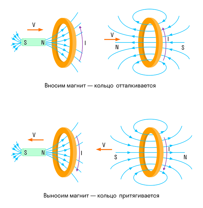
Давайте попробуем чуть проще: катушка в данном случае — это недовольная бабуля. Забирают у нее магнитный поток — она недовольна и создает магнитное поле, которое этот магнитный поток хочет обратно отобрать.

Дают ей магнитный поток, забирай, мол, пользуйся, а она такая — «Да зачем сдался мне ваш магнитный поток!» и создает магнитное поле, которое этот магнитный поток выгоняет.

Источник

Электромагнитная индукция

Содержание

Явление электромагнитной индукции
Магнитный поток
Закон электромагнитной индукции Фарадея
Правило Ленца
Самоиндукция
Индуктивность
Энергия магнитного поля
Основные формулы раздела «Электромагнитная индукция»

Явление электромагнитной индукции

Электромагнитная индукция – явление возникновения тока в замкнутом проводящем контуре при изменении магнитного потока, пронизывающего его.

Явление электромагнитной индукции было открыто М. Фарадеем.

Опыты Фарадея

На одну непроводящую основу были намотаны две катушки: витки первой катушки были расположены между витками второй. Витки одной катушки были замкнуты на гальванометр, а второй – подключены к источнику тока. При замыкании ключа и протекании тока по второй катушке в первой возникал импульс тока. При размыкании ключа также наблюдался импульс тока, но ток через гальванометр тек в противоположном направлении.
Первая катушка была подключена к источнику тока, вторая, подключенная к гальванометру, перемещалась относительно нее. При приближении или удалении катушки фиксировался ток.
Катушка замкнута на гальванометр, а магнит движется – вдвигается (выдвигается) – относительно катушки.

Опыты показали, что индукционный ток возникает только при изменении линий магнитной индукции. Направление тока будет различно при увеличении числа линий и при их уменьшении.

Сила индукционного тока зависит от скорости изменения магнитного потока. Может изменяться само поле, или контур может перемещаться в неоднородном магнитном поле.

Объяснения возникновения индукционного тока

Ток в цепи может существовать, когда на свободные заряды действуют сторонние силы. Работа этих сил по перемещению единичного положительного заряда вдоль замкнутого контура равна ЭДС. Значит, при изменении числа магнитных линий через поверхность, ограниченную контуром, в нем появляется ЭДС, которую называют ЭДС индукции.

Электроны в неподвижном проводнике могут приводиться в движение только электрическим полем. Это электрическое поле порождается изменяющимся во времени магнитным полем. Его называют вихревым электрическим полем. Представление о вихревом электрическом поле было введено в физику великим английским физиком Дж. Максвеллом в 1861 году.

Свойства вихревого электрического поля:

источник – переменное магнитное поле;
обнаруживается по действию на заряд;
не является потенциальным;
линии поля замкнутые.

Работа этого поля при перемещении единичного положительного заряда по замкнутому контуру равна ЭДС индукции в неподвижном проводнике.

Магнитный поток

Магнитным потоком через площадь ( S ) контура называют скалярную физическую величину, равную произведению модуля вектора магнитной индукции ( B ), площади поверхности ( S ), пронизываемой данным потоком, и косинуса угла ( alpha ) между направлением вектора магнитной индукции и вектора нормали (перпендикуляра к плоскости данной поверхности):

Обозначение – ( Phi ), единица измерения в СИ – вебер (Вб).

Магнитный поток в 1 вебер создается однородным магнитным полем с индукцией 1 Тл через поверхность площадью 1 м², расположенную перпендикулярно вектору магнитной индукции:

В зависимости от угла ( alpha ) магнитный поток может быть положительным (( alpha ) < 90°) или отрицательным (( alpha ) > 90°). Если ( alpha ) = 90°, то магнитный поток равен 0.

В случае неоднородного магнитного поля и неплоского контура магнитный поток находят как сумму магнитных потоков, пронизывающих площадь каждого из участков, на которые можно разбить данную поверхность.

Закон электромагнитной индукции Фарадея

Закон электромагнитной индукции (закон Фарадея):

ЭДС индукции в замкнутом контуре равна и противоположна по знаку скорости изменения магнитного потока через поверхность, ограниченную контуром:

Знак «–» в формуле позволяет учесть направление индукционного тока. Индукционный ток в замкнутом контуре имеет всегда такое направление, чтобы магнитный поток поля, созданного этим током сквозь поверхность, ограниченную контуром, уменьшал бы те изменения поля, которые вызвали появление индукционного тока.

Если контур состоит из ( N ) витков, то ЭДС индукции:

Сила индукционного тока в замкнутом проводящем контуре с сопротивлением ( R ):

При движении проводника длиной ( l ) со скоростью ( v ) в постоянном однородном магнитном поле с индукцией ( vec{B} ) ЭДС электромагнитной индукции равна:

где ( alpha ) – угол между векторами ( vec{B} ) и ( vec{v} ).

Важно!
Изменение магнитного потока, пронизывающего замкнутый контур, может происходить по двум причинам:

магнитный поток изменяется вследствие перемещения контура или его частей в постоянном во времени магнитном поле. Это случай, когда проводники, а вместе с ними и свободные носители заряда, движутся в магнитном поле;
вторая причина изменения магнитного потока, пронизывающего контур, – изменение во времени магнитного поля при неподвижном контуре. В этом случае возникновение ЭДС индукции уже нельзя объяснить действием силы Лоренца. Явление электромагнитной индукции в неподвижных проводниках, возникающее при изменении окружающего магнитного поля, также описывается формулой Фарадея.

в случае движущихся проводников ЭДС индукции обусловлена силой Лоренца;
в случае неподвижных проводников ЭДС индукции является следствием действия на свободные заряды вихревого электрического поля, возникающего при изменении магнитного поля.

Правило Ленца

Направление индукционного тока определяется по правилу Ленца: индукционный ток, возбуждаемый в замкнутом контуре при изменении магнитного потока, всегда направлен так, что создаваемое им магнитное поле препятствует изменению магнитного потока, вызывающего индукционный ток.

Алгоритм решения задач с использованием правила Ленца:

определить направление линий магнитной индукции внешнего магнитного поля;
выяснить, как изменяется магнитный поток;
определить направление линий магнитной индукции магнитного поля индукционного тока: если магнитный поток уменьшается, то они сонаправлены с линиями внешнего магнитного поля; если магнитный поток увеличивается, – противоположно направлению линий магнитной индукции внешнего поля;
по правилу буравчика, зная направление линий индукции магнитного поля индукционного тока, определить направление индукционного тока.

Правило Ленца имеет глубокий физический смысл – оно выражает закон сохранения энергии.

Самоиндукция

Самоиндукция – это явление возникновения ЭДС индукции в проводнике в результате изменения тока в нем.

При изменении силы тока в катушке происходит изменение магнитного потока, создаваемого этим током. Изменение магнитного потока, пронизывающего катушку, должно вызывать появление ЭДС индукции в катушке.

В соответствии с правилом Ленца ЭДС самоиндукции препятствует нарастанию силы тока при включении и убыванию силы тока при выключении цепи.

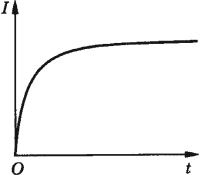
Это приводит к тому, что при замыкании цепи, в которой есть источник тока с постоянной ЭДС, сила тока устанавливается через некоторое время.

При отключении источника ток также не прекращается мгновенно. Возникающая при этом ЭДС самоиндукции может превышать ЭДС источника.

Явление самоиндукции можно наблюдать, собрав электрическую цепь из катушки с большой индуктивностью, резистора, двух одинаковых ламп накаливания и источника тока. Резистор должен иметь такое же электрическое сопротивление, как и провод катушки.

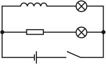
Опыт показывает, что при замыкании цепи электрическая лампа, включенная последовательно с катушкой, загорается несколько позже, чем лампа, включенная последовательно с резистором. Нарастанию тока в цепи катушки при замыкании препятствует ЭДС самоиндукции, возникающая при возрастании магнитного потока в катушке.

При отключении источника тока вспыхивают обе лампы. В этом случае ток в цепи поддерживается ЭДС самоиндукции, возникающей при убывании магнитного потока в катушке.

ЭДС самоиндукции ( varepsilon_{is} ), возникающая в катушке с индуктивностью ( L ), по закону электромагнитной индукции равна:

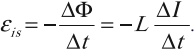
ЭДС самоиндукции прямо пропорциональна индуктивности катушки и скорости изменения силы тока в катушке.

Индуктивность

Электрический ток, проходящий по проводнику, создает вокруг него магнитное поле. Магнитный поток ( Phi ) через контур из этого проводника пропорционален модулю индукции ( vec{B} ) магнитного поля внутри контура, а индукция магнитного поля, в свою очередь, пропорциональна силе тока в проводнике.

Следовательно, магнитный поток через контур прямо пропорционален силе тока в контуре:

Индуктивность – коэффициент пропорциональности ( L ) между силой тока ( I ) в контуре и магнитным потоком ( Phi ), создаваемым этим током:

Индуктивность зависит от размеров и формы проводника, от магнитных свойств среды, в которой находится проводник.

Единица индуктивности в СИ – генри (Гн). Индуктивность контура равна 1 генри, если при силе постоянного тока 1 ампер магнитный поток через контур равен 1 вебер:

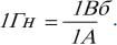
Можно дать второе определение единицы индуктивности: элемент электрической цепи обладает индуктивностью в 1 Гн, если при равномерном изменении силы тока в цепи на 1 ампер за 1 с в нем возникает ЭДС самоиндукции 1 вольт.

Энергия магнитного поля

При отключении катушки индуктивности от источника тока лампа накаливания, включенная параллельно катушке, дает кратковременную вспышку. Ток в цепи возникает под действием ЭДС самоиндукции.

Источником энергии, выделяющейся при этом в электрической цепи, является магнитное поле катушки.

Для создания тока в контуре с индуктивностью необходимо совершить работу на преодоление ЭДС самоиндукции. Энергия магнитного поля тока вычисляется по формуле:

Основные формулы раздела «Электромагнитная индукция»

Алгоритм решения задач по теме «Электромагнитная индукция»:

1. Внимательно прочитать условие задачи. Установить причины изменения магнитного потока, пронизывающего контур.

2. Записать формулу:

закона электромагнитной индукции;
ЭДС индукции в движущемся проводнике, если в задаче рассматривается поступательно движущийся проводник; если в задаче рассматривается электрическая цепь, содержащая источник тока, и возникающая на одном из участков ЭДС индукции, вызванная движением проводника в магнитном поле, то сначала нужно определить величину и направление ЭДС индукции. После этого задача решается по аналогии с задачами на расчет цепи постоянного тока с несколькими источниками.

3. Записать выражение для изменения магнитного потока и подставить в формулу закона электромагнитной индукции.

4. Записать математически все дополнительные условия (чаще всего это формулы закона Ома для полной цепи, силы Ампера или силы Лоренца, формулы кинематики и динамики).

5. Решить полученную систему уравнений относительно искомой величины.

6. Решение проверить.

Электромагнитная индукция

3.2 (63.8%) 79 votes

Источник

Магнитная индукция

Магнитная индукция — это силовая характеристика магнитного поля в выбранной точке пространства. Она определяет силу, с которой магнитное поле воздействует на заряженную частицу, что движется внутри него. Магнитная индукция считается фундаментальной характеристикой магнитного поля (как напряжённость для электрического поля).

Магнитная индукция описывает магнитную силу (вектор) на тестовом объекте (например, на куске железа) в каждой точке пространства. Простыми словами: если естественный магнит поднести к магнитным веществам (таким, как железо, никель, кобальт и т. д.), это вызовет в них магнитные свойства, которые называются «магнитной индукцией». Магнитная индукция используется для создания искусственных магнитов.

Магнитная индукция также называется плотностью магнитного потока.

Магнитная индукция измеряется:

в системе СИ единицей тесла (Тл),
в системе СГС единицей гаусс (Гс).

Соотношение между Тл и Гс: 1 Тл = 10 000 Гс.

Магнитная индукция — это векторная величина и обозначается буквой B со стрелочкой:

Индукция (от лат. inducere — вводить, наведение) — производство токов в цепи под действием магнита или другого тока.

Формулы вычисления магнитной индукции

Формула магнитной индукции:

Формула магнитной индукции: B = Mmax/IS

Где:

B — индукция магнитного поля (в Тл)
Mmax — максимальный крутящий момент магнитных сил, приложенных к рамке (в Нм)
l — длина проводника (в м)
S — площадь рамки (в м²)

Другие формулы, где встречается B

Эти формулы также можно использовать для её расчёта.

Сила Ампера:

Формулы вычисления магнитной индукции Fa=IBL sinα

Сила Ампера: Fa=IBL sinα

Где:

Fa — сила Ампера (в Н — ньютон)
I — сила тока (в А — ампер)
B — индукция магнитного поля (в Тл)
L — длина проводника (в м)
α — угол между вектором В и одним из направлений (силы тока, скорости или др.; измеряется в рад. или град.)

Сила Лоренца:

Формулы вычисления магнитной индукции Fл = qvB sinα

Сила Лоренца: Fл = qvB sinα

Где:

Fл — сила Лоренца (в Н — ньютон)
q — заряд частицы (в Кл — кулон)
v — скорость (в м/с)
B — индукция (в Тл)
α — угол между вектором В и одним из направлений (силы тока, скорости, или др.; измеряется в рад. или град.))

Магнитный поток:

Формулы вычисления магнитной индукции Ф = BS cosα

Магнитный поток: Ф = BS cosα

Где:

Ф — магнитный поток (в Вб — вебер)
B — индукция (в Тл)
S — площадь рамки (в м²)
α — угол между вектором В и одним из направлений (силы тока, скорости, или др.; измеряется в рад. или град.))

Электромагнитная индукция и магнитная индукция: какая между ними разница?

Электромагнитная индукция — это производство электродвижущей силы, создаваемой в результате относительного движения между магнитным полем и проводником.

Магнитная индукция может производить постоянный магнит, но может и не производить.

Электромагнитная индукция создаёт ток, но таким образом, что этот созданный ток противодействует изменению магнитного поля.

В электромагнитной индукции используются магниты и электрические цепи, а в магнитной индукции используются только магниты и магнитные материалы.

Узнайте также про:

Магнитное поле,
Магнитное поле Земли,
Уравнения Максвелла
Напряженность электрического поля.

Источник

Alternating electric current flows through the solenoid on the left, producing a changing magnetic field. This field causes, by electromagnetic induction, an electric current to flow in the wire loop on the right.

Electromagnetic or magnetic induction is the production of an electromotive force (emf) across an electrical conductor in a changing magnetic field.

Michael Faraday is generally credited with the discovery of induction in 1831, and James Clerk Maxwell mathematically described it as Faraday’s law of induction. Lenz’s law describes the direction of the induced field. Faraday’s law was later generalized to become the Maxwell–Faraday equation, one of the four Maxwell equations in his theory of electromagnetism.

Electromagnetic induction has found many applications, including electrical components such as inductors and transformers, and devices such as electric motors and generators.

History

Faraday’s experiment showing induction between coils of wire: The liquid battery (right) provides a current that flows through the small coil (A), creating a magnetic field. When the coils are stationary, no current is induced. But when the small coil is moved in or out of the large coil (B), the magnetic flux through the large coil changes, inducing a current which is detected by the galvanometer (G).^[1]

A diagram of Faraday’s iron ring apparatus. Change in the magnetic flux of the left coil induces a current in the right coil.^[2]

Electromagnetic induction was discovered by Michael Faraday, published in 1831.^[3]^[4] It was discovered independently by Joseph Henry in 1832.^[5]^[6]

In Faraday’s first experimental demonstration (August 29, 1831), he wrapped two wires around opposite sides of an iron ring or «torus» (an arrangement similar to a modern toroidal transformer).^{[citation needed]} Based on his understanding of electromagnets, he expected that, when current started to flow in one wire, a sort of wave would travel through the ring and cause some electrical effect on the opposite side. He plugged one wire into a galvanometer, and watched it as he connected the other wire to a battery. He saw a transient current, which he called a «wave of electricity», when he connected the wire to the battery and another when he disconnected it.^[7] This induction was due to the change in magnetic flux that occurred when the battery was connected and disconnected.^[2] Within two months, Faraday found several other manifestations of electromagnetic induction. For example, he saw transient currents when he quickly slid a bar magnet in and out of a coil of wires, and he generated a steady (DC) current by rotating a copper disk near the bar magnet with a sliding electrical lead («Faraday’s disk»).^[8]

Faraday explained electromagnetic induction using a concept he called lines of force. However, scientists at the time widely rejected his theoretical ideas, mainly because they were not formulated mathematically.^[9] An exception was James Clerk Maxwell, who used Faraday’s ideas as the basis of his quantitative electromagnetic theory.^[9]^[10]^[11] In Maxwell’s model, the time varying aspect of electromagnetic induction is expressed as a differential equation, which Oliver Heaviside referred to as Faraday’s law even though it is slightly different from Faraday’s original formulation and does not describe motional emf. Heaviside’s version (see Maxwell–Faraday equation below) is the form recognized today in the group of equations known as Maxwell’s equations.

In 1834 Heinrich Lenz formulated the law named after him to describe the «flux through the circuit». Lenz’s law gives the direction of the induced emf and current resulting from electromagnetic induction.

Theory

Faraday’s law of induction and Lenz’s law

The longitudinal cross section of a solenoid with a constant electrical current running through it. The magnetic field lines are indicated, with their direction shown by arrows. The magnetic flux corresponds to the ‘density of field lines’. The magnetic flux is thus densest in the middle of the solenoid, and weakest outside of it.

Faraday’s law of induction makes use of the magnetic flux Φ_B through a region of space enclosed by a wire loop. The magnetic flux is defined by a surface integral:^[12]

${displaystyle Phi _{mathrm {B} }=int _{Sigma }mathbf {B} cdot dmathbf {A} ,,}$

where dA is an element of the surface Σ enclosed by the wire loop, B is the magnetic field. The dot product B·dA corresponds to an infinitesimal amount of magnetic flux. In more visual terms, the magnetic flux through the wire loop is proportional to the number of magnetic field lines that pass through the loop.

When the flux through the surface changes, Faraday’s law of induction says that the wire loop acquires an electromotive force (emf).^{[note 1]} The most widespread version of this law states that the induced electromotive force in any closed circuit is equal to the rate of change of the magnetic flux enclosed by the circuit:^[16]^[17]

${displaystyle {mathcal {E}}=-{frac {dPhi _{mathrm {B} }}{dt}},,}$

where is the emf and Φ_B is the magnetic flux. The direction of the electromotive force is given by Lenz’s law which states that an induced current will flow in the direction that will oppose the change which produced it.^[18] This is due to the negative sign in the previous equation. To increase the generated emf, a common approach is to exploit flux linkage by creating a tightly wound coil of wire, composed of N identical turns, each with the same magnetic flux going through them. The resulting emf is then N times that of one single wire.^[19]^[20]

${displaystyle {mathcal {E}}=-N{frac {dPhi _{mathrm {B} }}{dt}}}$

Generating an emf through a variation of the magnetic flux through the surface of a wire loop can be achieved in several ways:

the magnetic field B changes (e.g. an alternating magnetic field, or moving a wire loop towards a bar magnet where the B field is stronger),
the wire loop is deformed and the surface Σ changes,
the orientation of the surface dA changes (e.g. spinning a wire loop into a fixed magnetic field),
any combination of the above

Maxwell–Faraday equation

In general, the relation between the emf in a wire loop encircling a surface Σ, and the electric field E in the wire is given by

${displaystyle {mathcal {E}}=oint _{partial Sigma }mathbf {E} cdot d{boldsymbol {ell }}}$

where dℓ is an element of contour of the surface Σ, combining this with the definition of flux

${displaystyle Phi _{mathrm {B} }=int _{Sigma }mathbf {B} cdot dmathbf {A} ,,}$

we can write the integral form of the Maxwell–Faraday equation

${displaystyle oint _{partial Sigma }mathbf {E} cdot d{boldsymbol {ell }}=-{frac {d}{dt}}{int _{Sigma }mathbf {B} cdot dmathbf {A} }}$

It is one of the four Maxwell’s equations, and therefore plays a fundamental role in the theory of classical electromagnetism.

Faraday’s law and relativity

Faraday’s law describes two different phenomena: the motional emf generated by a magnetic force on a moving wire (see Lorentz force), and the transformer emf this is generated by an electric force due to a changing magnetic field (due to the differential form of the Maxwell–Faraday equation). James Clerk Maxwell drew attention to the separate physical phenomena in 1861.^[21]^[22] This is believed to be a unique example in physics of where such a fundamental law is invoked to explain two such different phenomena.^[23]

Albert Einstein noticed that the two situations both corresponded to a relative movement between a conductor and a magnet, and the outcome was unaffected by which one was moving. This was one of the principal paths that led him to develop special relativity.^[24]

Applications

The principles of electromagnetic induction are applied in many devices and systems, including:

Current clamp
Electric generators
Electromagnetic forming
Graphics tablet
Hall effect sensors
Induction cooking
Induction motors
Induction sealing
Induction welding
Inductive charging
Inductors
Magnetic flow meters
Mechanically powered flashlight
Near-field communications
Pickups
Rowland ring
Transcranial magnetic stimulation
Transformers
Wireless energy transfer

Electrical generator

Rectangular wire loop rotating at angular velocity ω in radially outward pointing magnetic field B of fixed magnitude. The circuit is completed by brushes making sliding contact with top and bottom discs, which have conducting rims. This is a simplified version of the drum generator.

The emf generated by Faraday’s law of induction due to relative movement of a circuit and a magnetic field is the phenomenon underlying electrical generators. When a permanent magnet is moved relative to a conductor, or vice versa, an electromotive force is created. If the wire is connected through an electrical load, current will flow, and thus electrical energy is generated, converting the mechanical energy of motion to electrical energy. For example, the drum generator is based upon the figure to the bottom-right. A different implementation of this idea is the Faraday’s disc, shown in simplified form on the right.

In the Faraday’s disc example, the disc is rotated in a uniform magnetic field perpendicular to the disc, causing a current to flow in the radial arm due to the Lorentz force. Mechanical work is necessary to drive this current. When the generated current flows through the conducting rim, a magnetic field is generated by this current through Ampère’s circuital law (labelled «induced B» in the figure). The rim thus becomes an electromagnet that resists rotation of the disc (an example of Lenz’s law). On the far side of the figure, the return current flows from the rotating arm through the far side of the rim to the bottom brush. The B-field induced by this return current opposes the applied B-field, tending to decrease the flux through that side of the circuit, opposing the increase in flux due to rotation. On the near side of the figure, the return current flows from the rotating arm through the near side of the rim to the bottom brush. The induced B-field increases the flux on this side of the circuit, opposing the decrease in flux due to r the rotation. The energy required to keep the disc moving, despite this reactive force, is exactly equal to the electrical energy generated (plus energy wasted due to friction, Joule heating, and other inefficiencies). This behavior is common to all generators converting mechanical energy to electrical energy.

Electrical transformer

When the electric current in a loop of wire changes, the changing current creates a changing magnetic field. A second wire in reach of this magnetic field will experience this change in magnetic field as a change in its coupled magnetic flux, ${displaystyle {frac {dPhi _{B}}{dt}}}$ . Therefore, an electromotive force is set up in the second loop called the induced emf or transformer emf. If the two ends of this loop are connected through an electrical load, current will flow.

Current clamp

A current clamp is a type of transformer with a split core which can be spread apart and clipped onto a wire or coil to either measure the current in it or, in reverse, to induce a voltage. Unlike conventional instruments the clamp does not make electrical contact with the conductor or require it to be disconnected during attachment of the clamp.

Magnetic flow meter

Faraday’s law is used for measuring the flow of electrically conductive liquids and slurries. Such instruments are called magnetic flow meters. The induced voltage ε generated in the magnetic field B due to a conductive liquid moving at velocity v is thus given by:

where ℓ is the distance between electrodes in the magnetic flow meter.

Eddy currents

Electrical conductors moving through a steady magnetic field, or stationary conductors within a changing magnetic field, will have circular currents induced within them by induction, called eddy currents. Eddy currents flow in closed loops in planes perpendicular to the magnetic field. They have useful applications in eddy current brakes and induction heating systems. However eddy currents induced in the metal magnetic cores of transformers and AC motors and generators are undesirable since they dissipate energy (called core losses) as heat in the resistance of the metal. Cores for these devices use a number of methods to reduce eddy currents:

Cores of low frequency alternating current electromagnets and transformers, instead of being solid metal, are often made of stacks of metal sheets, called laminations, separated by nonconductive coatings. These thin plates reduce the undesirable parasitic eddy currents, as described below.
Inductors and transformers used at higher frequencies often have magnetic cores made of nonconductive magnetic materials such as ferrite or iron powder held together with a resin binder.

Electromagnet laminations

Eddy currents occur when a solid metallic mass is rotated in a magnetic field, because the outer portion of the metal cuts more magnetic lines of force than the inner portion; hence the induced electromotive force is not uniform; this tends to cause electric currents between the points of greatest and least potential. Eddy currents consume a considerable amount of energy and often cause a harmful rise in temperature.^[25]

Only five laminations or plates are shown in this example, so as to show the subdivision of the eddy currents. In practical use, the number of laminations or punchings ranges from 40 to 66 per inch (16 to 26 per centimetre), and brings the eddy current loss down to about one percent. While the plates can be separated by insulation, the voltage is so low that the natural rust/oxide coating of the plates is enough to prevent current flow across the laminations.^[25]

This is a rotor approximately 20 mm in diameter from a DC motor used in a CD player. Note the laminations of the electromagnet pole pieces, used to limit parasitic inductive losses.

Parasitic induction within conductors

In this illustration, a solid copper bar conductor on a rotating armature is just passing under the tip of the pole piece N of the field magnet. Note the uneven distribution of the lines of force across the copper bar. The magnetic field is more concentrated and thus stronger on the left edge of the copper bar (a,b) while the field is weaker on the right edge (c,d). Since the two edges of the bar move with the same velocity, this difference in field strength across the bar creates whorls or current eddies within the copper bar.^[25]

High current power-frequency devices, such as electric motors, generators and transformers, use multiple small conductors in parallel to break up the eddy flows that can form within large solid conductors. The same principle is applied to transformers used at higher than power frequency, for example, those used in switch-mode power supplies and the intermediate frequency coupling transformers of radio receivers.

References

Notes

^ The EMF is the voltage that would be measured by cutting the wire to create an open circuit, and attaching a voltmeter to the leads. Mathematically, is defined as the energy available from a unit charge that has traveled once around the wire loop.^[13]^[14]^[15]

References

^
Poyser, A. W. (1892). Magnetism and Electricity: A Manual for Students in Advanced Classes. London and New York: Longmans, Green, & Co. p. 285.
^ ^a ^b Giancoli, Douglas C. (1998). Physics: Principles with Applications (Fifth ed.). pp. 623–624.
^ Ulaby, Fawwaz (2007). Fundamentals of applied electromagnetics (5th ed.). Pearson:Prentice Hall. p. 255. ISBN 978-0-13-241326-8.
^ «Joseph Henry». Distinguished Members Gallery, National Academy of Sciences. Archived from the original on 2013-12-13. Retrieved 2006-11-30.
^ Errede, Steven (2007). «A Brief History of The Development of Classical Electrodynamics» (PDF).
^ «Electromagnetism». Smithsonian Institution Archives.
^ Michael Faraday, by L. Pearce Williams, p. 182–3
^ Michael Faraday, by L. Pearce Williams, p. 191–5
^ ^a ^b Michael Faraday, by L. Pearce Williams, p. 510
^ Maxwell, James Clerk (1904), A Treatise on Electricity and Magnetism, Vol. II, Third Edition. Oxford University Press, pp. 178–9 and 189.
^ «Archives Biographies: Michael Faraday», The Institution of Engineering and Technology.
^
Good, R. H. (1999). Classical Electromagnetism. Saunders College Publishing. p. 107. ISBN 0-03-022353-9.
^
Feynman, R. P.; Leighton, R. B.; Sands, M. L. (2006). The Feynman Lectures on Physics, Volume 2. Pearson/Addison-Wesley. p. 17-2. ISBN 0-8053-9049-9.
^
Griffiths, D. J. (1999). Introduction to Electrodynamics (3rd ed.). Prentice Hall. pp. 301–303. ISBN 0-13-805326-X.
^
Tipler, P. A.; Mosca, G. (2003). Physics for Scientists and Engineers (5th ed.). W.H. Freeman. p. 795. ISBN 978-0716708100.
^
Jordan, E.; Balmain, K. G. (1968). Electromagnetic Waves and Radiating Systems (2nd ed.). Prentice-Hall. p. 100. ISBN 9780132499958.
^
Hayt, W. (1989). Engineering Electromagnetics (5th ed.). McGraw-Hill. p. 312. ISBN 0-07-027406-1.
^
Schmitt, R. (2002). Electromagnetics Explained. Newnes. p. 75. ISBN 9780750674034.
^
Whelan, P. M.; Hodgeson, M. J. (1978). Essential Principles of Physics (2nd ed.). John Murray. ISBN 0-7195-3382-1.
^
Nave, C. R. «Faraday’s Law». HyperPhysics. Georgia State University. Retrieved 2011-08-29.
^
Maxwell, J. C. (1861). «On physical lines of force». Philosophical Magazine. 90 (139): 11–23. doi:10.1080/14786446108643033.
^
Griffiths, D. J. (1999). Introduction to Electrodynamics (3rd ed.). Prentice Hall. pp. 301–303. ISBN 0-13-805326-X. Note that the law relating flux to EMF, which this article calls «Faraday’s law», is referred to by Griffiths as the «universal flux rule». He uses the term «Faraday’s law» to refer to what this article calls the «Maxwell–Faraday equation».
^ «The flux rule» is the terminology that Feynman uses to refer to the law relating magnetic flux to EMF. Feynman, R. P.; Leighton, R. B.; Sands, M. L. (2006). The Feynman Lectures on Physics, Volume II. Pearson/Addison-Wesley. p. 17-2. ISBN 0-8053-9049-9.
^
Einstein, A. (1905). «Zur Elektrodynamik bewegter Körper» (PDF). Annalen der Physik. 17 (10): 891–921. Bibcode:1905AnP…322..891E. doi:10.1002/andp.19053221004.

Translated in Einstein, A. (1923). «On the Electrodynamics of Moving Bodies» (PDF). The Principle of Relativity. Jeffery, G.B.; Perret, W. (transl.). London: Methuen and Company.
^ ^a ^b ^c Images and reference text are from the public domain book: Hawkins Electrical Guide, Volume 1, Chapter 19: Theory of the Armature, pp. 270–273, Copyright 1917 by Theo. Audel & Co., Printed in the United States

External links

Media related to Electromagnetic induction at Wikimedia Commons
Tankersley and Mosca: Introducing Faraday’s law
A free java simulation on motional EMF

Источник

Electromagnetic or magnetic induction is the production of an electromotive force (emf) across an electrical conductor in a changing magnetic field.

Electromagnetic induction has found many applications, including electrical components such as inductors and transformers, and devices such as electric motors and generators.

History

A diagram of Faraday’s iron ring apparatus. Change in the magnetic flux of the left coil induces a current in the right coil.^[2]

Electromagnetic induction was discovered by Michael Faraday, published in 1831.^[3]^[4] It was discovered independently by Joseph Henry in 1832.^[5]^[6]

Theory

Faraday’s law of induction and Lenz’s law

Faraday’s law of induction makes use of the magnetic flux Φ_B through a region of space enclosed by a wire loop. The magnetic flux is defined by a surface integral:^[12]

${displaystyle Phi _{mathrm {B} }=int _{Sigma }mathbf {B} cdot dmathbf {A} ,,}$

${displaystyle {mathcal {E}}=-{frac {dPhi _{mathrm {B} }}{dt}},,}$

${displaystyle {mathcal {E}}=-N{frac {dPhi _{mathrm {B} }}{dt}}}$

Generating an emf through a variation of the magnetic flux through the surface of a wire loop can be achieved in several ways:

the magnetic field B changes (e.g. an alternating magnetic field, or moving a wire loop towards a bar magnet where the B field is stronger),
the wire loop is deformed and the surface Σ changes,
the orientation of the surface dA changes (e.g. spinning a wire loop into a fixed magnetic field),
any combination of the above