Определитель матрицы: алгоритм и примеры вычисления определителя матрицы
Определитель (детерминант) матрицы — некоторое число, с которым можно сопоставить любую квадратную матрицу А=(aij)n×n.
|А|, ∆, det A — символы, которыми обозначают определитель матрицы.
Способ вычисления определителя выбирают в зависимости от порядка матрицы.
Определитель матрицы 2-го порядка вычисляют по формуле:
А=1-231.
Решение:
det A=1-231=1×1-3×(-2)=1+6=7
Определитель матрицы 3-го порядка: правило треугольника
Чтобы найти определитель матрицы 3-го порядка, необходимо одно из правил:
- правило треугольника;
- правило Саррюса.
Как найти определитель матрицы 3-го порядка по методу треугольника?
а11а12а13а21а22а23а31а32а33=a11×a22×a33+a31×a12×a23+a21×a32×a13-a31×a22×a13-a21×a12×a33-a11×a23×a32
А=13402115-1
Решение:
det A=13402115-1=1×2×(-2)+1×3×1+4×0×5-1×2×4-0×3×(-1)-5×1×1=(-2)+3+0-8-0-5=-12
Правило Саррюса
Чтобы вычислить определитель по методу Саррюса, необходимо учесть некоторые условия и выполнить следующие действия:
- дописать слева от определителя два первых столбца;
- перемножить элементы, которые расположены на главной диагонали и параллельных ей диагоналях, взяв произведения со знаком «+»;
- перемножить элементы, которые расположены на побочных диагоналях и параллельных им, взяв произведения со знаком «—».
а11а12а13а21а22а23а31а32а33=a11×a22×a33+a31×a12×a23+a21×a32×a13-a31×a22×a13-a21×a12×a33-a11×a23×a32
А=134021-25-11302-25=1×2×(-1)+3×1×(-2)+4×0×5-4×2×(-2)-1×1×5-3×0×(-1)=-2-6+0+16-5-0=3
Методы разложения по элементам строки и столбца
Чтобы вычислить определитель матрицу 4-го порядка, можно воспользоваться одним из 2-х способов:
- разложением по элементам строки;
- разложением по элементам столбца.
Представленные способы определяют вычисление определителя n как вычисление определителя порядка n-1 за счет представления определителя суммой произведений элементов строки (столбца) на их алгебраические дополнения.
Разложение матрицы по элементам строки:
det A=ai1×Ai1+ai2×Ai2+…+аin×Аin
Разложение матрицы по элементам столбца:
det A=а1i×А1i+а2i×А2i+…+аni×Аni
Если раскладывать матрицу по элементам строки (столбца), необходимо выбирать строку (столбец), в которой(-ом) есть нули.
А=01-132100-24513210
Решение:
- раскладываем по 2-ой строке:
А=01-132100-24513210=2×(-1)3×1-13-251310=-2×1-13451210+1×0-13-251310
- раскладываем по 4-му столбцу:
А=01-132100-24513210=3×(-1)5×210-245321+1×(-1)7×01-1210321=-3×210-245321-1×01-1210321
Свойства определителя
Свойства определителя:
- если преобразовывать столбцы или строки незначительными действиями, то это не влияет на значение определителя;
- если поменять местами строки и столбцы, то знак поменяется на противоположный;
- определитель треугольной матрицы представляет собой произведение элементов, которые расположены на главной диагонали.
А=134021005
Решение:
det А=134021005=1×5×2=10
Определитель матрицы, который содержит нулевой столбец, равняется нулю.

Преподаватель математики и информатики. Кафедра бизнес-информатики Российского университета транспорта
Определитель матрицы и его свойства
8 февраля 2018
В этом уроке мы детально рассмотрим несколько ключевые вопросов и определений, благодаря чему вы раз и навсегда разберётесь и с матрицами, и с определителями, и со всеми их свойствами.
Определители — центральное понятие в алгебре матриц. Подобно формулам сокращённого умножения, они будут преследовать вас на протяжении всего курса высшей математики. Поэтому читаем, смотрим и разбираемся досконально.:)
И начнём мы с самого сокровенного — а что такое матрица? И как правильно с ней работать.
Правильная расстановка индексов в матрице
Матрица — это просто таблица, заполненная числами. Нео тут ни при чём.
Одна из ключевых характеристик матрицы — это её размерность, т.е. количество строк и столбцов, из которых она состоит. Обычно говорят, что некая матрица $A$ имеет размер $left[ mtimes n right]$, если в ней имеется $m$ строк и $n$ столбцов. Записывают это так:
[A=left[ mtimes n right]]
Или вот так:
[A=left( {{a}_{ij}} right),quad 1le ile m;quad 1le jle n.]
Бывают и другие обозначения — тут всё зависит от предпочтений лектора/ семинариста/ автора учебника. Но в любом случае со всеми этими $left[ mtimes n right]$ и ${{a}_{ij}}$ возникает одна и та же проблема:
Какой индекс за что отвечает? Сначала идёт номер строки, затем — столбца? Или наоборот?
При чтении лекций и учебников ответ будет казаться очевидным. Но когда на экзамене перед вами — только листик с задачей, можно переволноваться и внезапно запутаться.
Поэтому давайте разберёмся с этим вопросом раз и навсегда. Для начала вспомним обычную систему координат из школьного курса математики:
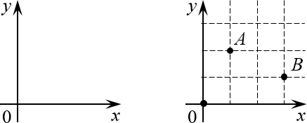
Помните её? У неё есть начало координат (точка $O=left( 0;0 right)$) оси $x$и $y$, а каждая точка на плоскости однозначно определяется по координатам: $A=left( 1;2 right)$, $B=left( 3;1 right)$ и т.д.
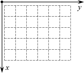
А теперь давайте возьмём эту конструкцию и поставим её рядом с матрицей так, чтобы начало координат находилось в левом верхнем углу. Почему именно там? Да потому что открывая книгу, мы начинаем читать именно с левого верхнего угла страницы — запомнить это легче лёгкого.
Но куда направить оси? Мы направим их так, чтобы вся наша виртуальная «страница» была охвачена этими осями. Правда, для этого придётся повернуть нашу систему координат. Единственно возможный вариант такого расположения:
Теперь всякая клетка матрицы имеет однозначные координаты $x$ и $y$. Например запись ${{a}_{24}}$ означает, что мы обращаемся к элементу с координатами $x=2$ и $y=4$. Размеры матрицы тоже однозначно задаются парой чисел:
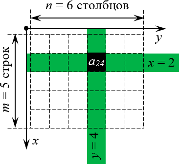
Просто всмотритесь в эту картинку внимательно. Поиграйтесь с координатами (особенно когда будете работать с настоящими матрицами и определителями) — и очень скоро поймёте, что даже в самых сложных теоремах и определениях вы прекрасно понимаете, о чём идёт речь.
Разобрались? Что ж, переходим к первому шагу просветления — геометрическому определению определителя.:)
Геометрическое определение
Прежде всего хотел бы отметить, что определитель существует только для квадратных матриц вида $left[ ntimes n right]$. Определитель — это число, которое cчитается по определённым правилам и является одной из характеристик этой матрицы (есть другие характеристики: ранг, собственные вектора, но об этом в других уроках).
Ну и что это за характеристика? Что он означает? Всё просто:
Определитель квадратной матрицы $A=left[ ntimes n right]$ — это объём $n$-мерного параллелепипеда, который образуется, если рассмотреть строки матрицы в качестве векторов, образующих рёбра этого параллелепипеда.
Например, определитель матрицы размера 2×2 — это просто площадь параллелограмма, а для матрицы 3×3 это уже объём 3-мерного параллелепипеда — того самого, который так бесит всех старшеклассников на уроках стереометрии.
На первый взгляд это определение может показаться совершенно неадекватным. Но давайте не будем спешить с выводами — глянем на примеры. На самом деле всё элементарно, Ватсон:
Задача. Найдите определители матриц:
[left| begin{matrix} 1 & 0 \ 0 & 3 \end{matrix} right|quad left| begin{matrix} 1 & -1 \ 2 & 2 \end{matrix} right|quad left| begin{matrix}2 & 0 & 0 \ 1 & 3 & 0 \ 1 & 1 & 4 \end{matrix} right|]
Решение. Первые два определителя имеют размер 2×2. Значит, это просто площади параллелограммов. Начертим их и посчитаем площадь.
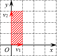
Первый параллелограмм построен на векторах ${{v}_{1}}=left( 1;0 right)$ и ${{v}_{2}}=left( 0;3 right)$:
Определитель 2×2 — это площадь параллелограмма Очевидно, это не просто параллелограмм, а вполне себе прямоугольник. Его площадь равна
[S=1cdot 3=3]
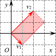
Второй параллелограмм построен на векторах ${{v}_{1}}=left( 1;-1 right)$ и ${{v}_{2}}=left( 2;2 right)$. Ну и что с того? Это тоже прямоугольник:
Ещё один определитель 2×2 Стороны этого прямоугольника (по сути — длины векторов) легко считаются по теореме Пифагора:
[begin{align} & left| {{v}_{1}} right|=sqrt{{{1}^{2}}+{{left( -1 right)}^{2}}}=sqrt{2}; \ & left| {{v}_{2}} right|=sqrt{{{2}^{2}}+{{2}^{2}}}=sqrt{8}=2sqrt{2}; \ & S=left| {{v}_{1}} right|cdot left| {{v}_{2}} right|=sqrt{2}cdot 2sqrt{2}=4. \end{align}]
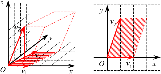
Осталось разобраться с последним определителем — там уже матрица 3×3. Придётся вспоминать стереометрию:
Определитель 3×3 — это объём параллелепипеда Выглядит мозговыносяще, но по факту достаточно вспомнить формулу объёма параллелепипеда:
[V=Scdot h]
где $S$ — площадь основания (в нашем случае это площадь параллелограмма на плоскости $OXY$), $h$ — высота, проведённая к этому основанию (по сути, $z$-координата вектора ${{v}_{3}}$).
Площадь параллелограмма (мы начертили его отдельно) тоже считается легко:
[begin{align} & S=2cdot 3=6; \ & V=Scdot h=6cdot 4=24. \end{align}]
Вот и всё! Записываем ответы.
Ответ: 3; 4; 24.
Небольшое замечание по поводу системы обозначений. Кому-то наверняка не понравится, что я игнорирую «стрелочки» над векторами. Якобы так можно спутать вектор с точкой или ещё с чем.
Но давайте серьёзно: мы с вами уже взрослые мальчики и девочки, поэтому из контекста прекрасно понимаем, когда речь идёт о векторе, а когда — о точке. Стрелки лишь засоряют повествование, и без того под завязку напичканное математическими формулами.
И ещё. В принципе, ничто не мешает рассмотреть и определитель матрицы 1×1 — такая матрица представляет собой просто одну клетку, а число, записанное в этой клетке, и будет определителем. Но тут есть важное замечание:
В отличие от классического объёма, определитель даст нам так называемый «ориентированный объём», т.е. объём с учётом последовательности рассмотрения векторов-строк.
И если вы хотите получить объём в классическом смысле этого слова, придётся взять модуль определителя, но сейчас не стоит париться об этом — всё равно через несколько секунд мы научимся считать любой определитель с любыми знаками, размерами и т.д.:)
Алгебраическое определение
При всей красоте и наглядности геометрического подхода у него есть серьёзный недостаток: он ничего не говорит нам о том, как этот самый определитель считать.
Поэтому сейчас мы разберём альтернативное определение — алгебраическое. Для этого нам потребуется краткая теоретическая подготовка, зато на выходе мы получим инструмент, позволяющий считать в матрицах что и как угодно.
Правда, там появится новая проблема… но обо всём по порядку.
Перестановки и инверсии
Давайте выпишем в строчку числа от 1 до $n$. Получится что-то типа этого:
[1;2;3;4;5;…;n-1;n]
Теперь (чисто по приколу) поменяем парочку чисел местами. Можно поменять соседние:
[1;3;2;4;5;…;n-1;n]
А можно — не особо соседние:
[n;2;3;4;5;…;n-1;1]
И знаете, что? А ничего! В алгебре эта хрень называется перестановкой. И у неё есть куча свойств.
Определение. Перестановка длины $n$ — строка из $n$ различных чисел, записанных в любой последовательности. Обычно рассматриваются первые $n$ натуральных чисел (т.е. как раз числа 1, 2, …, $n$), а затем их перемешивают для получения нужной перестановки.
Обозначаются перестановки так же, как и векторы — просто буквой и последовательным перечислением своих элементов в скобках. Например: $p=left( 1;3;2 right)$ или $p=left( 2;5;1;4;3 right)$. Буква может быть любой, но пусть будет $p$.:)
Далее для простоты изложения будем работать с перестановками длины 5 — они уже достаточно серьёзны для наблюдения всяких подозрительных эффектов, но ещё не настолько суровы для неокрепшего мозга, как перестановки длины 6 и более. Вот примеры таких перестановок:
[begin{align} & {{p}_{1}}=left( 1;2;3;4;5 right) \ & {{p}_{2}}=left( 1;3;2;5;4 right) \ & {{p}_{3}}=left( 5;4;3;2;1 right) \end{align}]
Естественно, перестановку длины $n$ можно рассматривать как функцию, которая определена на множестве $left{ 1;2;…;n right}$ и биективно отображает это множество на себя же. Возвращаясь к только что записанным перестановкам ${{p}_{1}}$, ${{p}_{2}}$ и ${{p}_{3}}$, мы вполне законно можем написать:
[{{p}_{1}}left( 1 right)=1;{{p}_{2}}left( 3 right)=2;{{p}_{3}}left( 2 right)=4;]
Количество различных перестановок длины $n$ всегда ограничено и равно $n!$ — это легко доказуемый факт из комбинаторики. Например, если мы захотим выписать все перестановки длины 5, то мы весьма заколебёмся, поскольку таких перестановок будет
[n!=5!=1cdot 2cdot 3cdot 4cdot 5=120]
Одной из ключевых характеристик всякой перестановки является количество инверсий в ней.
Определение. Инверсия в перестановке $p=left( {{a}_{1}};{{a}_{2}};…;{{a}_{n}} right)$ — всякая пара $left( {{a}_{i}};{{a}_{j}} right)$ такая, что $i lt j$, но ${{a}_{i}} gt {{a}_{j}}$. Проще говоря, инверсия — это когда большее число стоит левее меньшего (не обязательно соседнего).
Мы будем обозначать через $Nleft( p right)$ количество инверсий в перестановке $p$, но будьте готовы встретиться и с другими обозначениями в разных учебниках и у разных авторов — единых стандартов тут нет. Тема инверсий весьма обширна, и ей будет посвящён отдельный урок. Сейчас же наша задача — просто научиться считать их в реальных задачах.
Например, посчитаем количество инверсий в перестановке $p=left( 1;4;5;3;2 right)$:
[left( 4;3 right);left( 4;2 right);left( 5;3 right);left( 5;2 right);left( 3;2 right).]
Таким образом, $Nleft( p right)=5$. Как видите, ничего страшного в этом нет. Сразу скажу: дальше нас будет интересовать не столько само число $Nleft( p right)$, сколько его чётность/ нечётность. И тут мы плавно переходим к ключевому термину сегодняшнего урока.
Что такое определитель
Пусть дана квадратная матрица $A=left[ ntimes n right]$. Тогда:
Определение. Определитель матрицы $A=left[ ntimes n right]$ — это алгебраическая сумма $n!$ слагаемых, составленных следующим образом. Каждое слагаемое — это произведение $n$ элементов матрицы, взятых по одному из каждой строки и каждого столбца, умноженное на (−1) в степени количество инверсий:
[left| A right|=sumlimits_{n!}{{{left( -1 right)}^{Nleft( p right)}}cdot {{a}_{1;pleft( 1 right)}}cdot {{a}_{2;pleft( 2 right)}}cdot …cdot {{a}_{n;pleft( n right)}}}]
Принципиальным моментом при выборе множителей для каждого слагаемого в определителе является тот факт, что никакие два множителя не стоят в одной строчке или в одном столбце.
Благодаря этому можно без ограничения общности считать, что индексы $i$ множителей ${{a}_{i;j}}$ «пробегают» значения 1, …, $n$, а индексы $j$ являются некоторой перестановкой от первых:
[j=pleft( i right),quad i=1,2,…,n]
А когда есть перестановка $p$, мы легко посчитаем инверсии $Nleft( p right)$ — и очередное слагаемое определителя готово.
Естественно, никто не запрещает поменять местами множители в каком-либо слагаемом (или во всех сразу — чего мелочиться-то?), и тогда первые индексы тоже будут представлять собой некоторую перестановку. Но в итоге ничего не поменяется: суммарное количество инверсий в индексах $i$ и $j$ сохраняет чётность при подобных извращениях, что вполне соответствует старому-доброму правилу:
От перестановки множителей произведение чисел не меняется.
Вот только не надо приплетать это правило к умножению матриц — в отличие от умножения чисел, оно не коммутативно. Но это я отвлёкся.:)
Матрица 2×2
Вообще-то можно рассмотреть и матрицу 1×1 — это будет одна клетка, и её определитель, как нетрудно догадаться, равен числу, записанному в этой клетке. Ничего интересного.
Поэтому давайте рассмотрим квадратную матрицу размером 2×2:
[left[ begin{matrix} {{a}_{11}} & {{a}_{12}} \ {{a}_{21}} & {{a}_{22}} \end{matrix} right]]
Поскольку количество строк в ней $n=2$, то определитель будет содержать $n!=2!=1cdot 2=2$ слагаемых. Выпишем их:
[begin{align} & {{left( -1 right)}^{Nleft( 1;2 right)}}cdot {{a}_{11}}cdot {{a}_{22}}={{left( -1 right)}^{0}}cdot {{a}_{11}}cdot {{a}_{22}}={{a}_{11}}{{a}_{22}}; \ & {{left( -1 right)}^{Nleft( 2;1 right)}}cdot {{a}_{12}}cdot {{a}_{21}}={{left( -1 right)}^{1}}cdot {{a}_{12}}cdot {{a}_{21}}={{a}_{12}}{{a}_{21}}. \end{align}]
Очевидно, что в перестановке $left( 1;2 right)$, состоящей из двух элементов, нет инверсий, поэтому $Nleft( 1;2 right)=0$. А вот в перестановке $left( 2;1 right)$ одна инверсия имеется (собственно, 2 < 1), поэтому $Nleft( 2;1 right)=1.$
Итого универсальная формула вычисления определителя для матрицы 2×2 выглядит так:
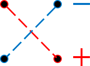
[left| begin{matrix} {{a}_{11}} & {{a}_{12}} \ {{a}_{21}} & {{a}_{22}} \end{matrix} right|={{a}_{11}}{{a}_{22}}-{{a}_{12}}{{a}_{21}}]
Графически это можно представить как произведение элементов, стоящих на главной диагонали, минус произведение элементов на побочной:
Рассмотрим пару примеров:
Задача. Вычислите определитель:
[left| begin{matrix} 5 & 6 \ 8 & 9 \end{matrix} right|;quad left| begin{matrix} 7 & 12 \ 14 & 1 \end{matrix} right|.]
Решение. Всё считается в одну строчку. Первая матрица:
[5cdot 9-8cdot 6=45-48=-3]
И вторая:
[7cdot 1-14cdot 12=7-168=-161]
Ответ: −3; −161.
Впрочем, это было слишком просто. Давайте рассмотрим матрицы 3×3 — там уже интересно.
Матрица 3×3
Теперь рассмотрим квадратную матрицу размера 3×3:
[left[ begin{matrix} {{a}_{11}} & {{a}_{12}} & {{a}_{13}} \ {{a}_{21}} & {{a}_{22}} & {{a}_{23}} \ {{a}_{31}} & {{a}_{32}} & {{a}_{33}} \end{matrix} right]]
При вычислении её определителя мы получим $3!=1cdot 2cdot 3=6$ слагаемых — ещё не слишком много для паники, но уже достаточно, чтобы начать искать какие-то закономерности. Для начала выпишем все перестановки из трёх элементов и посчитаем инверсии в каждой из них:
[begin{align} & {{p}_{1}}=left( 1;2;3 right)Rightarrow Nleft( {{p}_{1}} right)=Nleft( 1;2;3 right)=0; \ & {{p}_{2}}=left( 1;3;2 right)Rightarrow Nleft( {{p}_{2}} right)=Nleft( 1;3;2 right)=1; \ & {{p}_{3}}=left( 2;1;3 right)Rightarrow Nleft( {{p}_{3}} right)=Nleft( 2;1;3 right)=1; \ & {{p}_{4}}=left( 2;3;1 right)Rightarrow Nleft( {{p}_{4}} right)=Nleft( 2;3;1 right)=2; \ & {{p}_{5}}=left( 3;1;2 right)Rightarrow Nleft( {{p}_{5}} right)=Nleft( 3;1;2 right)=2; \ & {{p}_{6}}=left( 3;2;1 right)Rightarrow Nleft( {{p}_{6}} right)=Nleft( 3;2;1 right)=3. \end{align}]
Как и предполагалось, всего выписано 6 перестановок ${{p}_{1}}$, … ${{p}_{6}}$ (естественно, можно было бы выписать их в другой последовательности — суть от этого не изменится), а количество инверсий в них меняется от 0 до 3.
В общем, у нас будет три слагаемых с «плюсом» (там, где $Nleft( p right)$ — чётное) и ещё три с «минусом». А в целом определитель будет считаться по формуле:
[left| begin{matrix} {{a}_{11}} & {{a}_{12}} & {{a}_{13}} \ {{a}_{21}} & {{a}_{22}} & {{a}_{23}} \ {{a}_{31}} & {{a}_{32}} & {{a}_{33}} \end{matrix} right|=begin{matrix} {{a}_{11}}{{a}_{22}}{{a}_{33}}+{{a}_{12}}{{a}_{23}}{{a}_{31}}+{{a}_{13}}{{a}_{21}}{{a}_{32}}- \ -{{a}_{13}}{{a}_{22}}{{a}_{31}}-{{a}_{12}}{{a}_{21}}{{a}_{33}}-{{a}_{11}}{{a}_{23}}{{a}_{32}} \end{matrix}]
Вот только не надо сейчас садиться и яростно зубрить все эти индексы! Вместо непонятных цифр лучше запомните следующее мнемоническое правило:
Правило треугольника. Для нахождения определителя матрицы 3×3 нужно сложить три произведения элементов, стоящих на главной диагонали и в вершинах равнобедренных треугольников со стороной, параллельной этой диагонали, а затем вычесть такие же три произведения, но на побочной диагонали. Схематически это выглядит так:
Определитель матрицы 3×3: правило треугольников
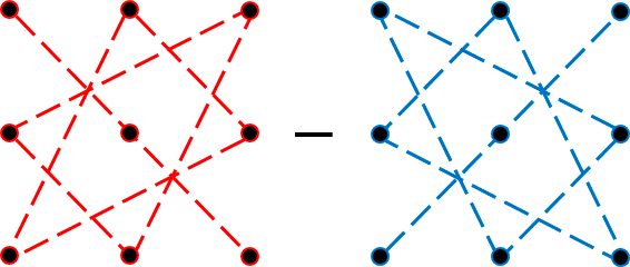
Именно эти треугольники (или пентаграммы — кому как больше нравится) любят рисовать во всяких учебниках и методичках по алгебре. Впрочем, не будем о грустном. Давайте лучше посчитаем один такой определитель — для разминки перед настоящей жестью.:)
Задача. Вычислите определитель:
[left| begin{matrix} 1 & 2 & 3 \ 4 & 5 & 6 \ 7 & 8 & 1 \end{matrix} right|]
Решение. Работаем по правилу треугольников. Сначала посчитаем три слагаемых, составленных из элементов на главной диагонали и параллельно ей:
[begin{align} & 1cdot 5cdot 1+2cdot 6cdot 7+3cdot 4cdot 8= \ & =5+84+96=185 \end{align}]
Теперь разбираемся с побочной диагональю:
[begin{align} & 3cdot 5cdot 7+2cdot 4cdot 1+1cdot 6cdot 8= \ & =105+8+48=161 \end{align}]
Осталось лишь вычесть из первого числа второе — и мы получим ответ:
[185-161=24]
Вот и всё!
Ответ: 24.
Тем не менее, определители матриц 3×3 — это ещё не вершина мастерства. Самое интересное ждёт нас дальше.:)
Общая схема вычисления определителей
Как мы знаем, с ростом размерности матрицы $n$ количество слагаемых в определителе составляет $n!$ и быстро растёт. Всё-таки факториал — это вам не хрен собачий довольно быстро растущая функция.
Уже для матриц 4×4 считать определители напролом (т.е. через перестановки) становится как-то не оч. Про 5×5 и более вообще молчу. Поэтому к делу подключаются некоторые свойства определителя, но для их понимания нужна небольшая теоретическая подготовка.
Готовы? Поехали!
Что такое минор матрицы
Пусть дана произвольная матрица $A=left[ mtimes n right]$. Заметьте: не обязательно квадратная. В отличие от определителей, миноры — это такие няшки, которые существуют не только в суровых квадратных матрицах. Выберем в этой матрице несколько (например, $k$) строк и столбцов, причём $1le kle m$ и $1le kle n$. Тогда:
Определение. Минор порядка $k$ — определитель квадратной матрицы, возникающей на пересечении выбранных $k$ столбцов и строк. Также минором мы будем называть и саму эту новую матрицу.
Обозначается такой минор ${{M}_{k}}$. Естественно, у одной матрицы может быть целая куча миноров порядка $k$. Вот пример минора порядка 2 для матрицы $left[ 5times 6 right]$:
Выбор $k = 2$ столбцов и строк для формирования минора
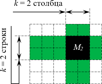
Совершенно необязательно, чтобы выбранные строки и столбцы стояли рядом, как в рассмотренном примере. Главное, чтобы количество выбранных строк и столбцов было одинаковым (это и есть число $k$).
Есть и другое определение. Возможно, кому-то оно больше придётся по душе:
Определение. Пусть дана прямоугольная матрица $A=left[ mtimes n right]$. Если после вычеркивания в ней одного или нескольких столбцов и одной или нескольких строк образуется квадратная матрица размера $left[ ktimes k right]$, то её определитель — это и есть минор ${{M}_{k}}$. Саму матрицу мы тоже иногда будем называть минором — это будет ясно из контекста.
Как говорил мой кот, иногда лучше один раз навернуться с 11-го этажа есть корм, чем мяукать, сидя на балконе.
Пример. Пусть дана матрица
[A=left[ begin{matrix} begin{matrix} 1 \ 2 \ 3 \end{matrix} & begin{matrix} 7 \ 4 \ 0 \end{matrix} & begin{matrix} 9 \ 5 \ 6 \end{matrix} & begin{matrix} 0 \ 3 \ 1 \end{matrix} \end{matrix} right]]
Выбирая строку 1 и столбец 2, получаем минор первого порядка:
[{{M}_{1}}=left| 7 right|=7]
Выбирая строки 2, 3 и столбцы 3, 4, получаем минор второго порядка:
[{{M}_{2}}=left| begin{matrix} 5 & 3 \ 6 & 1 \end{matrix} right|=5-18=-13]
А если выбрать все три строки, а также столбцы 1, 2, 4, будет минор третьего порядка:
[{{M}_{3}}=left| begin{matrix} 1 & 7 & 0 \ 2 & 4 & 3 \ 3 & 0 & 1 \end{matrix} right|]
Считать этот определитель мне уже в лом. Но он равен 53.:)
Читателю не составит труда найти и другие миноры порядков 1, 2 или 3. Поэтому идём дальше.
Алгебраические дополнения
«Ну ok, и что дают нам эти миньоны миноры?» — наверняка спросите вы. Сами по себе — ничего. Но в квадратных матрицах у каждого минора появляется «компаньон» — дополнительный минор, а также алгебраическое дополнение. И вместе эти два ушлёпка позволят нам щёлкать определители как орешки.
Определение. Пусть дана квадратная матрица $A=left[ ntimes n right]$, в которой выбран минор ${{M}_{k}}$. Тогда дополнительный минор для минора ${{M}_{k}}$ — это кусок исходной матрицы $A$, который останется при вычёркивании всех строк и столбцов, задействованных при составлении минора ${{M}_{k}}$:
Дополнительный минор к минору ${{M}_{2}}$ Уточним один момент: дополнительный минор — это не просто «кусок матрицы», а определитель этого куска.
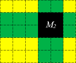
Обозначаются дополнительные миноры с помощью «звёздочки»: $M_{k}^{*}$:
[M_{k}^{*}=left| Anabla {{M}_{k}} right|]
где операция $Anabla {{M}_{k}}$ буквально означает «вычеркнуть из $A$ строки и столбцы, входящие в ${{M}_{k}}$». Эта операция не является общепринятой в математике — я её сам только что придумал для красоты повествования.:)
Дополнительные миноры редко используются сами по себе. Они являются частью более сложной конструкции — алгебраического дополнения.
Определение. Алгебраическое дополнение минора ${{M}_{k}}$ — это дополнительный минор $M_{k}^{*}$, умноженный на величину ${{left( -1 right)}^{S}}$, где $S$ — сумма номеров всех строк и столбцов, задействованных в исходном миноре ${{M}_{k}}$.
Как правило, алгебраическое дополнение минора ${{M}_{k}}$ обозначается через ${{A}_{k}}$. Поэтому:
[{{A}_{k}}={{left( -1 right)}^{S}}cdot M_{k}^{*}]
Сложно? На первый взгляд — да. Но это не точно. Потому что на самом деле всё легко. Рассмотрим пример:
Пример. Дана матрица 4×4:
[A=left[ begin{matrix} 1 & 2 & 3 & 4 \ 5 & 6 & 7 & 8 \ 9 & 10 & 11 & 12 \ 13 & 14 & 15 & 16 \end{matrix} right]]
Выберем минор второго порядка
[{{M}_{2}}=left| begin{matrix} 3 & 4 \ 15 & 16 \end{matrix} right|]
Капитан Очевидность как бы намекает нам, что при составлении этого минора были задействованы строки 1 и 4, а также столбцы 3 и 4. Вычёркиваем их — получим дополнительный минор:
[M_{2}^{*}=left| begin{matrix} 5 & 6 \ 9 & 10 \end{matrix} right|=50-54=-4]
Осталось найти число $S$ и получить алгебраическое дополнение. Поскольку мы знаем номера задействованных строк (1 и 4) и столбцов (3 и 4), всё просто:
[begin{align} & S=1+4+3+4=12; \ & {{A}_{2}}={{left( -1 right)}^{S}}cdot M_{2}^{*}={{left( -1 right)}^{12}}cdot left( -4 right)=-4end{align}]
Ответ: ${{A}_{2}}=-4$
Вот и всё! По сути, всё различие между дополнительным минором и алгебраическим дополнением — только в минусе спереди, да и то не всегда.
Наша задача сейчас — научиться быстро считать алгебраические дополнения, потому что они являются составной частью «Теоремы, Которую Нельзя Называть». Но мы всё же назовём. Встречайте:
Теорема Лапласа
И вот мы пришли к тому, зачем, собственно, все эти миноры и алгебраические дополнения были нужны.
Теорема Лапласа о разложении определителя. Пусть в матрице размера $left[ ntimes n right]$ выбрано $k$ строк (столбцов), причём $1le kle n-1$. Тогда определитель этой матрицы равен сумме всех произведений миноров порядка $k$, содержащихся в выбранных строках (столбцах), на их алгебраические дополнения:
[left| A right|=sum{{{M}_{k}}cdot {{A}_{k}}}]
Причём таких слагаемых будет ровно $C_{n}^{k}$.
Ладно, ладно: про $C_{n}^{k}$ — это я уже понтуюсь, в оригинальной теореме Лапласа ничего такого не было. Но комбинаторику никто не отменял, и буквально беглый взгляд на условие позволит вам самостоятельно убедиться, что слагаемых будет именно столько.:)
Мы не будем её доказывать, хоть это и не представляет особой трудности — все выкладки сводятся к старым-добрым перестановкам и чётности/ нечётности инверсий. Тем не менее, доказательство будет представлено в отдельном параграфе, а сегодня у нас сугубо практический урок.
Поэтому переходим к частному случаю этой теоремы, когда миноры представляют собой отдельные клетки матрицы.
Разложение определителя по строке и столбцу
То, о чём сейчас пойдёт речь — как раз и есть основной инструмент работы с определителями, ради которого затевались вся эта дичь с перестановками, минорами и алгебраическими дополнениями.
Читайте и наслаждайтесь:
Следствие из Теоремы Лапласа (разложение определителя по строке/столбцу). Пусть в матрице размера $left[ ntimes n right]$ выбрана одна строка. Минорами в этой строке будут $n$ отдельных клеток:
[{{M}_{1}}={{a}_{ij}},quad j=1,…,n]
Дополнительные миноры тоже легко считаются: просто берём исходную матрицу и вычёркиваем строку и столбец, содержащие ${{a}_{ij}}$. Назовём такие миноры $M_{ij}^{*}$.
Для алгебраического дополнения ещё нужно число $S$, но в случае с минором порядка 1 это просто сумма «координат» клетки ${{a}_{ij}}$:
[S=i+j]
И тогда исходный определитель можно расписать через ${{a}_{ij}}$ и $M_{ij}^{*}$ согласно теореме Лапласа:
[left| A right|=sumlimits_{j=1}^{n}{{{a}_{ij}}cdot {{left( -1 right)}^{i+j}}cdot {{M}_{ij}}}]
Это и есть формула разложения определителя по строке. Но то же верно и для столбцов.
Из этого следствия можно сразу сформулировать несколько выводов:
- Эта схема одинаково хорошо работает как для строк, так и для столбцов. На самом деле чаще всего разложение будет идти именно по столбцам, нежели по строкам.
- Количество слагаемых в разложении всегда ровно $n$. Это существенно меньше $C_{n}^{k}$ и уж тем более $n!$.
- Вместо одного определителя $left[ ntimes n right]$ придётся считать несколько определителей размера на единицу меньше: $left[ left( n-1 right)times left( n-1 right) right]$.
Последний факт особенно важен. Например, вместо зверского определителя 4×4 теперь достаточно будет посчитать несколько определителей 3×3 — с ними мы уж как-нибудь справимся.:)
Что ж, попробуем посчитать одну такую задачку?
Задача. Найдите определитель:
[left| begin{matrix} 1 & 2 & 3 \ 4 & 5 & 6 \ 7 & 8 & 9 \end{matrix} right|]
Решение. Разложим этот определитель по первой строке:
[begin{align} left| A right|=1cdot {{left( -1 right)}^{1+1}}cdot left| begin{matrix} 5 & 6 \ 8 & 9 \end{matrix} right|+ & \ 2cdot {{left( -1 right)}^{1+2}}cdot left| begin{matrix} 4 & 6 \ 7 & 9 \end{matrix} right|+ & \ 3cdot {{left( -1 right)}^{1+3}}cdot left| begin{matrix} 4 & 5 \ 7 & 8 \end{matrix} right|= & \end{align}]
[begin{align} & =1cdot left( 45-48 right)-2cdot left( 36-42 right)+3cdot left( 32-35 right)= \ & =1cdot left( -3 right)-2cdot left( -6 right)+3cdot left( -3 right)=0. \end{align}]
Ответ: 0.
Задача. Найдите определитель:
[left| begin{matrix} 0 & 1 & 1 & 0 \ 1 & 0 & 1 & 1 \ 1 & 1 & 0 & 1 \ 1 & 1 & 1 & 0 \end{matrix} right|]
Решение. Для разнообразия давайте в этот раз работать со столбцами. Например, в последнем столбце присутствуют сразу два нуля — очевидно, это значительно сократит вычисления. Сейчас увидите почему.
Итак, раскладываем определитель по четвёртому столбцу:
[begin{align} left| begin{matrix} 0 & 1 & 1 & 0 \ 1 & 0 & 1 & 1 \ 1 & 1 & 0 & 1 \ 1 & 1 & 1 & 0 \end{matrix} right|=0cdot {{left( -1 right)}^{1+4}}cdot left| begin{matrix} 1 & 0 & 1 \ 1 & 1 & 0 \ 1 & 1 & 1 \end{matrix} right|+ & \ +1cdot {{left( -1 right)}^{2+4}}cdot left| begin{matrix} 0 & 1 & 1 \ 1 & 1 & 0 \ 1 & 1 & 1 \end{matrix} right|+ & \ +1cdot {{left( -1 right)}^{3+4}}cdot left| begin{matrix} 0 & 1 & 1 \ 1 & 0 & 1 \ 1 & 1 & 1 \end{matrix} right|+ & \ +0cdot {{left( -1 right)}^{4+4}}cdot left| begin{matrix} 0 & 1 & 1 \ 1 & 0 & 1 \ 1 & 1 & 0 \end{matrix} right| & \end{align}]
И тут — о, чудо! — два слагаемых сразу улетают коту под хвост, поскольку в них есть множитель «0». Остаётся ещё два определителя 3×3, с которыми мы легко разберёмся:
[begin{align} & left| begin{matrix} 0 & 1 & 1 \ 1 & 1 & 0 \ 1 & 1 & 1 \end{matrix} right|=0+0+1-1-1-0=-1; \ & left| begin{matrix} 0 & 1 & 1 \ 1 & 0 & 1 \ 1 & 1 & 1 \end{matrix} right|=0+1+1-0-0-1=1. \end{align}]
Возвращаемся к исходнику и находим ответ:
[left| begin{matrix} 0 & 1 & 1 & 0 \ 1 & 0 & 1 & 1 \ 1 & 1 & 0 & 1 \ 1 & 1 & 1 & 0 \end{matrix} right|=1cdot left( -1 right)+left( -1 right)cdot 1=-2]
Ну вот и всё. И никаких 4! = 24 слагаемых считать не пришлось.:)
Ответ: −2
Основные свойства определителя
В последней задаче мы видели, как наличие нулей в строках (столбцах) матрицы резко упрощает разложение определителя и вообще все вычисления. Возникает естественный вопрос: а нельзя ли сделать так, чтобы эти нули появились даже в той матрице, где их изначально не было?
Ответ однозначен: можно. И здесь нам на помощь приходят свойства определителя:
- Если поменять две строчки (столбца) местами, определитель поменяет знак;
- Если одну строку (столбец) умножить на число $k$, то весь определитель тоже умножится на число $k$;
- Если взять одну строку и прибавить (вычесть) её сколько угодно раз из другой, определитель не изменится;
- Если две строки определителя одинаковы, либо пропорциональны, либо одна из строк заполнена нулями, то весь определитель равен нулю;
- Все указанные выше свойства верны и для столбцов.
- При транспонировании матрицы определитель не меняется;
- Определитель произведения матриц равен произведению определителей.
Особую ценность представляет третье свойство: мы можем вычитать из одной строки (столбца) другую до тех пор, пока в нужных местах не появятся нули.
Чаще всего расчёты сводится к тому, чтобы «обнулить» весь столбец везде, кроме одного элемента, а затем разложить определитель по этому столбцу, получив матрицу размером на 1 меньше.
Давайте посмотрим, как это работает на практике:
Задача. Найдите определитель:
[left| begin{matrix} 1 & 2 & 3 & 4 \ 4 & 1 & 2 & 3 \ 3 & 4 & 1 & 2 \ 2 & 3 & 4 & 1 \end{matrix} right|]
Решение. Нулей тут как бы вообще не наблюдается, поэтому можно «долбить» по любой строке или столбцу — объём вычислений будет примерно одинаковым. Давайте не будем мелочиться и «обнулим» первый столбец: в нём уже есть клетка с единицей, поэтому просто возьмём первую строчку и вычтем её 4 раза из второй, 3 раза из третьей и 2 раза из последней.
В результате мы получим новую матрицу, но её определитель будет тем же:
[begin{matrix} left| begin{matrix} 1 & 2 & 3 & 4 \ 4 & 1 & 2 & 3 \ 3 & 4 & 1 & 2 \ 2 & 3 & 4 & 1 \end{matrix} right|begin{matrix} downarrow \ -4 \ -3 \ -2 \end{matrix}= \ =left| begin{matrix} 1 & 2 & 3 & 4 \ 4-4cdot 1 & 1-4cdot 2 & 2-4cdot 3 & 3-4cdot 4 \ 3-3cdot 1 & 4-3cdot 2 & 1-3cdot 3 & 2-3cdot 4 \ 2-2cdot 1 & 3-2cdot 2 & 4-2cdot 3 & 1-2cdot 4 \end{matrix} right|= \ =left| begin{matrix} 1 & 2 & 3 & 4 \ 0 & -7 & -10 & -13 \ 0 & -2 & -8 & -10 \ 0 & -1 & -2 & -7 \end{matrix} right| \end{matrix}]
Теперь с невозмутимостью Пятачка раскладываем этот определитель по первому столбцу:
[begin{matrix} 1cdot {{left( -1 right)}^{1+1}}cdot left| begin{matrix} -7 & -10 & -13 \ -2 & -8 & -10 \ -1 & -2 & -7 \end{matrix} right|+0cdot {{left( -1 right)}^{2+1}}cdot left| … right|+ \ +0cdot {{left( -1 right)}^{3+1}}cdot left| … right|+0cdot {{left( -1 right)}^{4+1}}cdot left| … right| \end{matrix}]
Понятно, что «выживет» только первое слагаемое — в остальных я даже определители не выписывал, поскольку они всё равно умножаются на ноль. Коэффициент перед определителем равен единице, т.е. его можно не записывать.
Зато можно вынести «минусы» из всех трёх строк определителя. По сути, мы трижды вынесли множитель (−1):
[left| begin{matrix} -7 & -10 & -13 \ -2 & -8 & -10 \ -1 & -2 & -7 \end{matrix} right|=cdot left| begin{matrix} 7 & 10 & 13 \ 2 & 8 & 10 \ 1 & 2 & 7 \end{matrix} right|]
Получили мелкий определитель 3×3, который уже можно посчитать по правилу треугольников. Но мы попробуем разложить и его по первому столбцу — благо в последней строчке гордо стоит единица:
[begin{align} & left( -1 right)cdot left| begin{matrix} 7 & 10 & 13 \ 2 & 8 & 10 \ 1 & 2 & 7 \end{matrix} right|begin{matrix} -7 \ -2 \ uparrow \end{matrix}=left( -1 right)cdot left| begin{matrix} 0 & -4 & -36 \ 0 & 4 & -4 \ 1 & 2 & 7 \end{matrix} right|= \ & =cdot left| begin{matrix} -4 & -36 \ 4 & -4 \end{matrix} right|=left( -1 right)cdot left| begin{matrix} -4 & -36 \ 4 & -4 \end{matrix} right| \end{align}]
Можно, конечно, ещё поприкалываться и разложить матрицу 2×2 по строке (столбцу), но мы же с вами адекватны, поэтому просто посчитаем ответ:
[left( -1 right)cdot left| begin{matrix} -4 & -36 \ 4 & -4 \end{matrix} right|=left( -1 right)cdot left( 16+144 right)=-160]
Вот так и разбиваются мечты. Всего-то −160 в ответе.:)
Ответ: −160.
Парочка замечаний перед тем, как мы перейдём к последней задаче:
- Исходная матрица была симметрична относительно побочной диагонали. Все миноры в разложении тоже симметричны относительно той же побочной диагонали.
- Строго говоря, мы могли вообще ничего не раскладывать, а просто привести матрицу к верхнетреугольному виду, когда под главной диагональю стоят сплошные нули. Тогда (в точном соответствии с геометрической интерпретацией, кстати) определитель равен произведению ${{a}_{ii}}$ — чисел на главной диагонали.
Идём дальше. Последняя задача в сегодняшнем уроке.
Задача. Найдите определитель:
[left| begin{matrix} 1 & 1 & 1 & 1 \ 2 & 4 & 8 & 16 \ 3 & 9 & 27 & 81 \ 5 & 25 & 125 & 625 \end{matrix} right|]
Решение. Ну, тут первая строка прямо-таки напрашивается на «обнуление». Берём первый столбец и вычитаем ровно один раз из всех остальных:
[begin{align} & left| begin{matrix} 1 & 1 & 1 & 1 \ 2 & 4 & 8 & 16 \ 3 & 9 & 27 & 81 \ 5 & 25 & 125 & 625 \end{matrix} right|= \ & =left| begin{matrix} 1 & 1-1 & 1-1 & 1-1 \ 2 & 4-2 & 8-2 & 16-2 \ 3 & 9-3 & 27-3 & 81-3 \ 5 & 25-5 & 125-5 & 625-5 \end{matrix} right|= \ & =left| begin{matrix} 1 & 0 & 0 & 0 \ 2 & 2 & 6 & 14 \ 3 & 6 & 24 & 78 \ 5 & 20 & 120 & 620 \end{matrix} right| \end{align}]
Раскладываем по первой строке, а затем выносим общие множители из оставшихся строк:
[cdot left| begin{matrix} 2 & 6 & 14 \ 6 & 24 & 78 \ 20 & 120 & 620 \end{matrix} right|=cdot left| begin{matrix} 1 & 3 & 7 \ 1 & 4 & 13 \ 1 & 6 & 31 \end{matrix} right|]
Снова наблюдаем «красивые» числа, но уже в первом столбце — раскладываем определитель по нему:
[begin{align} & 240cdot left| begin{matrix} 1 & 3 & 7 \ 1 & 4 & 13 \ 1 & 6 & 31 \end{matrix} right|begin{matrix} downarrow \ -1 \ -1 \end{matrix}=240cdot left| begin{matrix} 1 & 3 & 7 \ 0 & 1 & 6 \ 0 & 3 & 24 \end{matrix} right|= \ & =240cdot {{left( -1 right)}^{1+1}}cdot left| begin{matrix} 1 & 6 \ 3 & 24 \end{matrix} right|= \ & =240cdot 1cdot left( 24-18 right)=1440 \end{align}]
Порядок. Задача решена.
Ответ: 1440
Всё. Хорош читать этот бред.:)
Смотрите также:
- Обратная матрица

- Умножение матриц

- Геометрическая вероятность
- Решение задач B12: №448—455
- Задачи на проценты: формула, упрощающая вычисления
- Задача B4 про три дороги — стандартная задача на движение
This article is about mathematics. For determinants in epidemiology, see Risk factor. For determinants in immunology, see Epitope.
In mathematics, the determinant is a scalar value that is a function of the entries of a square matrix. It characterizes some properties of the matrix and the linear map represented by the matrix. In particular, the determinant is nonzero if and only if the matrix is invertible and the linear map represented by the matrix is an isomorphism. The determinant of a product of matrices is the product of their determinants (the preceding property is a corollary of this one).
The determinant of a matrix A is denoted det(A), det A, or |A|.
The determinant of a 2 × 2 matrix is

and the determinant of a 3 × 3 matrix is

The determinant of a n × n matrix can be defined in several equivalent ways. Leibniz formula expresses the determinant as a sum of signed products of matrix entries such that each summand is the product of n different entries, and the number of these summands is  the factorial of n (the product of the n first positive integers). The Laplace expansion expresses the determinant of a n × n matrix as a linear combination of determinants of
  submatrices. Gaussian elimination express the determinant as the product of the diagonal entries of a diagonal matrix that is obtained by a succession of elementary row operations.
Determinants can also be defined by some of their properties: the determinant is the unique function defined on the n × n matrices that has the four following properties. The determinant of the identity matrix is 1; the exchange of two rows (or of two columns) multiplies the determinant by −1; multiplying a row (or a column) by a number multiplies the determinant by this number; and adding to a row (or a column) a multiple of another row (or column) does not change the determinant.
Determinants occur throughout mathematics. For example, a matrix is often used to represent the coefficients in a system of linear equations, and determinants can be used to solve these equations (Cramer’s rule), although other methods of solution are computationally much more efficient. Determinants are used for defining the characteristic polynomial of a matrix, whose roots are the eigenvalues. In geometry, the signed n-dimensional volume of a n-dimensional parallelepiped is expressed by a determinant. This is used in calculus with exterior differential forms and the Jacobian determinant, in particular for changes of variables in multiple integrals.
2 × 2 matrices[edit]
The determinant of a 2 × 2 matrix  is denoted either by «det» or by vertical bars around the matrix, and is defined as

For example,

First properties[edit]
The determinant has several key properties that can be proved by direct evaluation of the definition for  -matrices, and that continue to hold for determinants of larger matrices. They are as follows:[1] first, the determinant of the identity matrix
  is 1.
is 1.
Second, the determinant is zero if two rows are the same:

This holds similarly if the two columns are the same. Moreover,

Finally, if any column is multiplied by some number  (i.e., all entries in that column are multiplied by that number), the determinant is also multiplied by that number:

Geometric meaning[edit]
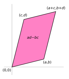
The area of the parallelogram is the absolute value of the determinant of the matrix formed by the vectors representing the parallelogram’s sides.
If the matrix entries are real numbers, the matrix A can be used to represent two linear maps: one that maps the standard basis vectors to the rows of A, and one that maps them to the columns of A. In either case, the images of the basis vectors form a parallelogram that represents the image of the unit square under the mapping. The parallelogram defined by the rows of the above matrix is the one with vertices at (0, 0), (a, b), (a + c, b + d), and (c, d), as shown in the accompanying diagram.
The absolute value of ad − bc is the area of the parallelogram, and thus represents the scale factor by which areas are transformed by A. (The parallelogram formed by the columns of A is in general a different parallelogram, but since the determinant is symmetric with respect to rows and columns, the area will be the same.)
The absolute value of the determinant together with the sign becomes the oriented area of the parallelogram. The oriented area is the same as the usual area, except that it is negative when the angle from the first to the second vector defining the parallelogram turns in a clockwise direction (which is opposite to the direction one would get for the identity matrix).
To show that ad − bc is the signed area, one may consider a matrix containing two vectors u ≡ (a, b) and v ≡ (c, d) representing the parallelogram’s sides. The signed area can be expressed as |u| |v| sin θ for the angle θ between the vectors, which is simply base times height, the length of one vector times the perpendicular component of the other. Due to the sine this already is the signed area, yet it may be expressed more conveniently using the cosine of the complementary angle to a perpendicular vector, e.g. u⊥ = (−b, a), so that |u⊥| |v| cos θ′, which can be determined by the pattern of the scalar product to be equal to ad − bc:

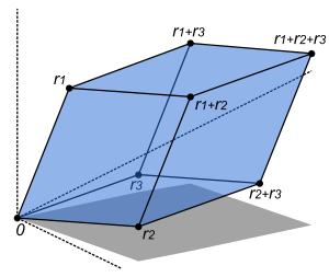
The volume of this parallelepiped is the absolute value of the determinant of the matrix formed by the columns constructed from the vectors r1, r2, and r3.
Thus the determinant gives the scaling factor and the orientation induced by the mapping represented by A. When the determinant is equal to one, the linear mapping defined by the matrix is equi-areal and orientation-preserving.
The object known as the bivector is related to these ideas. In 2D, it can be interpreted as an oriented plane segment formed by imagining two vectors each with origin (0, 0), and coordinates (a, b) and (c, d). The bivector magnitude (denoted by (a, b) ∧ (c, d)) is the signed area, which is also the determinant ad − bc.[2]
If an n × n real matrix A is written in terms of its column vectors ![{displaystyle A=left[{begin{array}{c|c|c|c}mathbf {a} _{1}&mathbf {a} _{2}&cdots &mathbf {a} _{n}end{array}}right]}](https://wikimedia.org/api/rest_v1/media/math/render/svg/b1d60337c4cde7b2d5fc3e0365bc8ec5e699ea1a) , then
, then

This means that  maps the unit n-cube to the n-dimensional parallelotope defined by the vectors
  the region
The determinant gives the signed n-dimensional volume of this parallelotope,  and hence describes more generally the n-dimensional volume scaling factor of the linear transformation produced by A.[3] (The sign shows whether the transformation preserves or reverses orientation.) In particular, if the determinant is zero, then this parallelotope has volume zero and is not fully n-dimensional, which indicates that the dimension of the image of A is less than n. This means that A produces a linear transformation which is neither onto nor one-to-one, and so is not invertible.
Definition[edit]
In the sequel, A is a square matrix with n rows and n columns, so that it can be written as

The entries  etc. are, for many purposes, real or complex numbers. As discussed below, the determinant is also defined for matrices whose entries are in a commutative ring.
The determinant of A is denoted by det(A), or it can be denoted directly in terms of the matrix entries by writing enclosing bars instead of brackets:

There are various equivalent ways to define the determinant of a square matrix A, i.e. one with the same number of rows and columns: the determinant can be defined via the Leibniz formula, an explicit formula involving sums of products of certain entries of the matrix. The determinant can also be characterized as the unique function depending on the entries of the matrix satisfying certain properties. This approach can also be used to compute determinants by simplifying the matrices in question.
Leibniz formula[edit]
3 × 3 matrices[edit]
The Leibniz formula for the determinant of a 3 × 3 matrix is the following:

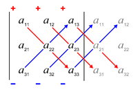
The rule of Sarrus is a mnemonic for the expanded form of this determinant: the sum of the products of three diagonal north-west to south-east lines of matrix elements, minus the sum of the products of three diagonal south-west to north-east lines of elements, when the copies of the first two columns of the matrix are written beside it as in the illustration. This scheme for calculating the determinant of a 3 × 3 matrix does not carry over into higher dimensions.
n × n matrices[edit]
In higher dimension, the Leibniz formula expresses the determinant of an  -matrix as an expression involving permutations and their signatures. A permutation of the set
  is a function
  that reorders this set of integers. The value in the
  -th position after the reordering is denoted below by
  . The set of all such permutations, called the symmetric group, is commonly denoted
  . The signature
  of a permutation is
  if the permutation can be obtained with an even number of exchanges of two entries; otherwise, it is
Given a matrix

the Leibniz formula for its determinant is, using sigma notation,

Using pi notation, this can be shortened into
 .
.

The Levi-Civita symbol  is defined on the n-tuples of integers in
  as 0 if two of the integers are equal, and, otherwise, as the signature of the permutation defined by the tuple of integers. With the Levi-Civita symbol, Leibniz formula may be written as

where the sum is taken over all n-tuples of integers in 
[4][5]
Properties of the determinant[edit]
Characterization of the determinant[edit]
The determinant can be characterized by the following three key properties. To state these, it is convenient to regard an -matrix A as being composed of its  columns, so denoted as

where the column vector  (for each i) is composed of the entries of the matrix in the i-th column.
- , where is an identity matrix.
- The determinant is multilinear: if the jth column of a matrix is written as a linear combination of two column vectors v and w and a number r, then the determinant of A is expressible as a similar linear combination:
- The determinant is alternating: whenever two columns of a matrix are identical, its determinant is 0:


If the determinant is defined using the Leibniz formula as above, these three properties can be proved by direct inspection of that formula. Some authors also approach the determinant directly using these three properties: it can be shown that there is exactly one function that assigns to any -matrix A a number that satisfies these three properties.[6] This also shows that this more abstract approach to the determinant yields the same definition as the one using the Leibniz formula.
To see this it suffices to expand the determinant by multi-linearity in the columns into a (huge) linear combination of determinants of matrices in which each column is a standard basis vector. These determinants are either 0 (by property 9) or else ±1 (by properties 1 and 12 below), so the linear combination gives the expression above in terms of the Levi-Civita symbol. While less technical in appearance, this characterization cannot entirely replace the Leibniz formula in defining the determinant, since without it the existence of an appropriate function is not clear.[citation needed]
Immediate consequences[edit]
These rules have several further consequences:
- The determinant is a homogeneous function, i.e.,
(for an
matrix ). - Interchanging any pair of columns of a matrix multiplies its determinant by −1. This follows from the determinant being multilinear and alternating (properties 2 and 3 above):
This formula can be applied iteratively when several columns are swapped. For example
Yet more generally, any permutation of the columns multiplies the determinant by the sign of the permutation.
- If some column can be expressed as a linear combination of the other columns (i.e. the columns of the matrix form a linearly dependent set), the determinant is 0. As a special case, this includes: if some column is such that all its entries are zero, then the determinant of that matrix is 0.
- Adding a scalar multiple of one column to another column does not change the value of the determinant. This is a consequence of multilinearity and being alternative: by multilinearity the determinant changes by a multiple of the determinant of a matrix with two equal columns, which determinant is 0, since the determinant is alternating.
- If is a triangular matrix, i.e. , whenever or, alternatively, whenever , then its determinant equals the product of the diagonal entries:
Indeed, such a matrix can be reduced, by appropriately adding multiples of the columns with fewer nonzero entries to those with more entries, to a diagonal matrix (without changing the determinant). For such a matrix, using the linearity in each column reduces to the identity matrix, in which case the stated formula holds by the very first characterizing property of determinants. Alternatively, this formula can also be deduced from the Leibniz formula, since the only permutation
which gives a non-zero contribution is the identity permutation.


Example[edit]
These characterizing properties and their consequences listed above are both theoretically significant, but can also be used to compute determinants for concrete matrices. In fact, Gaussian elimination can be applied to bring any matrix into upper triangular form, and the steps in this algorithm affect the determinant in a controlled way. The following concrete example illustrates the computation of the determinant of the matrix using that method:

| Matrix |  |
|
|
|
| Obtained by |
add the second column to the first |
add 3 times the third column to the second |
swap the first two columns |
add |
| Determinant |  |
|
|
|


Combining these equalities gives 
Transpose[edit]
The determinant of the transpose of equals the determinant of A:
- .

This can be proven by inspecting the Leibniz formula.[7] This implies that in all the properties mentioned above, the word «column» can be replaced by «row» throughout. For example, viewing an n × n matrix as being composed of n rows, the determinant is an n-linear function.
Multiplicativity and matrix groups[edit]
The determinant is a multiplicative map, i.e., for square matrices and  of equal size, the determinant of a matrix product equals the product of their determinants:

This key fact can be proven by observing that, for a fixed matrix , both sides of the equation are alternating and multilinear as a function depending on the columns of . Moreover, they both take the value  when is the identity matrix. The above-mentioned unique characterization of alternating multilinear maps therefore shows this claim.[8]
A matrix is invertible precisely if its determinant is nonzero. This follows from the multiplicativity of  and the formula for the inverse involving the adjugate matrix mentioned below. In this event, the determinant of the inverse matrix is given by
- .
![{displaystyle det left(A^{-1}right)={frac {1}{det(A)}}=[det(A)]^{-1}}](https://wikimedia.org/api/rest_v1/media/math/render/svg/f4f6798a0a88679c1b82126428cf67aae28244fc)
In particular, products and inverses of matrices with non-zero determinant (respectively, determinant one) still have this property. Thus, the set of such matrices (of fixed size ) forms a group known as the general linear group  (respectively, a subgroup called the special linear group
  . More generally, the word «special» indicates the subgroup of another matrix group of matrices of determinant one. Examples include the special orthogonal group (which if n is 2 or 3 consists of all rotation matrices), and the special unitary group.
The Cauchy–Binet formula is a generalization of that product formula for rectangular matrices. This formula can also be recast as a multiplicative formula for compound matrices whose entries are the determinants of all quadratic submatrices of a given matrix.[9][10]
Laplace expansion[edit]
Laplace expansion expresses the determinant of a matrix in terms of determinants of smaller matrices, known as its minors. The minor  is defined to be the determinant of the -matrix that results from by removing the -th row and the
  -th column. The expression
  is known as a cofactor. For every , one has the equality

which is called the Laplace expansion along the ith row. For example, the Laplace expansion along the first row ( ) gives the following formula:

Unwinding the determinants of these -matrices gives back the Leibniz formula mentioned above. Similarly, the Laplace expansion along the -th column is the equality

Laplace expansion can be used iteratively for computing determinants, but this approach is inefficient for large matrices. However, it is useful for computing the determinants of highly symmetric matrix such as the Vandermonde matrix

This determinant has been applied, for example, in the proof of Baker’s theorem in the theory of transcendental numbers.
Adjugate matrix[edit]
The adjugate matrix  is the transpose of the matrix of the cofactors, that is,

For every matrix, one has[11]

Thus the adjugate matrix can be used for expressing the inverse of a nonsingular matrix:

Block matrices[edit]
The formula for the determinant of a -matrix above continues to hold, under appropriate further assumptions, for a block matrix, i.e., a matrix composed of four submatrices  of dimension ,
  ,
,  and
and  , respectively. The easiest such formula, which can be proven using either the Leibniz formula or a factorization involving the Schur complement, is

If is invertible (and similarly if  is invertible[12]), one has

If is a  -matrix, this simplifies to
  .
.
If the blocks are square matrices of the same size further formulas hold. For example, if  and commute (i.e.,
  ), then there holds [13]

This formula has been generalized to matrices composed of more than blocks, again under appropriate commutativity conditions among the individual blocks.[14]
For  and
and  , the following formula holds (even if and do not commute)[citation needed]

Sylvester’s determinant theorem[edit]
Sylvester’s determinant theorem states that for A, an m × n matrix, and B, an n × m matrix (so that A and B have dimensions allowing them to be multiplied in either order forming a square matrix):

where Im and In are the m × m and n × n identity matrices, respectively.
From this general result several consequences follow.
Sum[edit]
The determinant of the sum  of two square matrices of the same size is not in general expressible in terms of the determinants of A and of B. However, for positive semidefinite matrices , and of equal size,

with the corollary[16][17]

Conversely, if and are Hermitian, positive-definite, and size , then the determinant has concave th root;[18] this implies
![{displaystyle {sqrt[{n}]{det {!(A+B)}}}geq {sqrt[{n}]{det {!(A)}}}+{sqrt[{n}]{det {!(B)}}}}](https://wikimedia.org/api/rest_v1/media/math/render/svg/8e77020a4af805fa2f6e3d5b1a1eaab10c936bcb)
by homogeneity.
Sum identity for 2×2 matrices[edit]
For the special case of matrices with complex entries, the determinant of the sum can be written in terms of determinants and traces in the following identity:

Proof of identity
This can be shown by writing out each term in components  . The left-hand side is

Expanding gives

The terms which are quadratic in are seen to be  , and similarly for , so the expression can be written

We can then write the cross-terms as

which can be recognized as

which completes the proof.
This has an application to matrix algebras. For example, consider the complex numbers as a matrix algebra. The complex numbers have a representation as matrices of the form

with  and
and  real. Since
  , taking
  and
and  in the above identity gives

This result followed just from and  .
.
Properties of the determinant in relation to other notions[edit]
Eigenvalues and characteristic polynomial[edit]
The determinant is closely related to two other central concepts in linear algebra, the eigenvalues and the characteristic polynomial of a matrix. Let be an -matrix with complex entries with eigenvalues  . (Here it is understood that an eigenvalue with algebraic multiplicity μ occurs μ times in this list.) Then the determinant of A is the product of all eigenvalues,

The product of all non-zero eigenvalues is referred to as pseudo-determinant.
The characteristic polynomial is defined as[19]

Here,  is the indeterminate of the polynomial and
  is the identity matrix of the same size as . By means of this polynomial, determinants can be used to find the eigenvalues of the matrix : they are precisely the roots of this polynomial, i.e., those complex numbers
  such that

A Hermitian matrix is positive definite if all its eigenvalues are positive. Sylvester’s criterion asserts that this is equivalent to the determinants of the submatrices

being positive, for all  between
  and .[20]
Trace[edit]
The trace tr(A) is by definition the sum of the diagonal entries of A and also equals the sum of the eigenvalues. Thus, for complex matrices A,

or, for real matrices A,

Here exp(A) denotes the matrix exponential of A, because every eigenvalue λ of A corresponds to the eigenvalue exp(λ) of exp(A). In particular, given any logarithm of A, that is, any matrix L satisfying

the determinant of A is given by

For example, for n = 2, n = 3, and n = 4, respectively,

cf. Cayley-Hamilton theorem. Such expressions are deducible from combinatorial arguments, Newton’s identities, or the Faddeev–LeVerrier algorithm. That is, for generic n, detA = (−1)nc0 the signed constant term of the characteristic polynomial, determined recursively from

In the general case, this may also be obtained from[21]

where the sum is taken over the set of all integers kl ≥ 0 satisfying the equation

The formula can be expressed in terms of the complete exponential Bell polynomial of n arguments sl = −(l – 1)! tr(Al) as

This formula can also be used to find the determinant of a matrix AIJ with multidimensional indices I = (i1, i2, …, ir) and J = (j1, j2, …, jr). The product and trace of such matrices are defined in a natural way as

An important arbitrary dimension n identity can be obtained from the Mercator series expansion of the logarithm when the expansion converges. If every eigenvalue of A is less than 1 in absolute value,

where I is the identity matrix. More generally, if

is expanded as a formal power series in s then all coefficients of sm for m > n are zero and the remaining polynomial is det(I + sA).
Upper and lower bounds[edit]
For a positive definite matrix A, the trace operator gives the following tight lower and upper bounds on the log determinant

with equality if and only if A = I. This relationship can be derived via the formula for the Kullback-Leibler divergence between two multivariate normal distributions.
Also,

These inequalities can be proved by expressing the traces and the determinant in terms of the eigenvalues. As such, they represent the well-known fact that the harmonic mean is less than the geometric mean, which is less than the arithmetic mean, which is, in turn, less than the root mean square.
Derivative[edit]
The Leibniz formula shows that the determinant of real (or analogously for complex) square matrices is a polynomial function from  to
to  . In particular, it is everywhere differentiable. Its derivative can be expressed using Jacobi’s formula:[22]

where denotes the adjugate of . In particular, if is invertible, we have

Expressed in terms of the entries of , these are

Yet another equivalent formulation is
- ,

using big O notation. The special case where  , the identity matrix, yields

This identity is used in describing Lie algebras associated to certain matrix Lie groups. For example, the special linear group  is defined by the equation
  . The above formula shows that its Lie algebra is the special linear Lie algebra
  consisting of those matrices having trace zero.
Writing a  -matrix as
  where
where  are column vectors of length 3, then the gradient over one of the three vectors may be written as the cross product of the other two:

History[edit]
Historically, determinants were used long before matrices: A determinant was originally defined as a property of a system of linear equations.
The determinant «determines» whether the system has a unique solution (which occurs precisely if the determinant is non-zero).
In this sense, determinants were first used in the Chinese mathematics textbook The Nine Chapters on the Mathematical Art (九章算術, Chinese scholars, around the 3rd century BCE). In Europe, solutions of linear systems of two equations were expressed by Cardano in 1545 by a determinant-like entity.[23]
Determinants proper originated from the work of Seki Takakazu in 1683 in Japan and parallelly of Leibniz in 1693.[24][25][26][27] Cramer (1750) stated, without proof, Cramer’s rule.[28] Both Cramer and also Bezout (1779) were led to determinants by the question of plane curves passing through a given set of points.[29]
Vandermonde (1771) first recognized determinants as independent functions.[25] Laplace (1772) gave the general method of expanding a determinant in terms of its complementary minors: Vandermonde had already given a special case.[30] Immediately following, Lagrange (1773) treated determinants of the second and third order and applied it to questions of elimination theory; he proved many special cases of general identities.
Gauss (1801) made the next advance. Like Lagrange, he made much use of determinants in the theory of numbers. He introduced the word «determinant» (Laplace had used «resultant»), though not in the present signification, but rather as applied to the discriminant of a quantic.[31] Gauss also arrived at the notion of reciprocal (inverse) determinants, and came very near the multiplication theorem.
The next contributor of importance is Binet (1811, 1812), who formally stated the theorem relating to the product of two matrices of m columns and n rows, which for the special case of m = n reduces to the multiplication theorem. On the same day (November 30, 1812) that Binet presented his paper to the Academy, Cauchy also presented one on the subject. (See Cauchy–Binet formula.) In this he used the word «determinant» in its present sense,[32][33] summarized and simplified what was then known on the subject, improved the notation, and gave the multiplication theorem with a proof more satisfactory than Binet’s.[25][34] With him begins the theory in its generality.
(Jacobi 1841) used the functional determinant which Sylvester later called the Jacobian.[35] In his memoirs in Crelle’s Journal for 1841 he specially treats this subject, as well as the class of alternating functions which Sylvester has called alternants. About the time of Jacobi’s last memoirs, Sylvester (1839) and Cayley began their work. Cayley 1841 introduced the modern notation for the determinant using vertical bars.[36][37]
The study of special forms of determinants has been the natural result of the completion of the general theory. Axisymmetric determinants have been studied by Lebesgue, Hesse, and Sylvester; persymmetric determinants by Sylvester and Hankel; circulants by Catalan, Spottiswoode, Glaisher, and Scott; skew determinants and Pfaffians, in connection with the theory of orthogonal transformation, by Cayley; continuants by Sylvester; Wronskians (so called by Muir) by Christoffel and Frobenius; compound determinants by Sylvester, Reiss, and Picquet; Jacobians and Hessians by Sylvester; and symmetric gauche determinants by Trudi. Of the textbooks on the subject Spottiswoode’s was the first. In America, Hanus (1886), Weld (1893), and Muir/Metzler (1933) published treatises.
Applications[edit]
Cramer’s rule[edit]
Determinants can be used to describe the solutions of a linear system of equations, written in matrix form as  . This equation has a unique solution
  if and only if is nonzero. In this case, the solution is given by Cramer’s rule:

where  is the matrix formed by replacing the -th column of by the column vector . This follows immediately by column expansion of the determinant, i.e.

where the vectors  are the columns of A. The rule is also implied by the identity

Cramer’s rule can be implemented in  time, which is comparable to more common methods of solving systems of linear equations, such as LU, QR, or singular value decomposition.[38]
Linear independence[edit]
Determinants can be used to characterize linearly dependent vectors:  is zero if and only if the column vectors (or, equivalently, the row vectors) of the matrix are linearly dependent.[39] For example, given two linearly independent vectors
  , a third vector
  lies in the plane spanned by the former two vectors exactly if the determinant of the -matrix consisting of the three vectors is zero. The same idea is also used in the theory of differential equations: given functions
  (supposed to be
  times differentiable), the Wronskian is defined to be

It is non-zero (for some ) in a specified interval if and only if the given functions and all their derivatives up to order are linearly independent. If it can be shown that the Wronskian is zero everywhere on an interval then, in the case of analytic functions, this implies the given functions are linearly dependent. See the Wronskian and linear independence. Another such use of the determinant is the resultant, which gives a criterion when two polynomials have a common root.[40]
Orientation of a basis[edit]
The determinant can be thought of as assigning a number to every sequence of n vectors in Rn, by using the square matrix whose columns are the given vectors. For instance, an orthogonal matrix with entries in Rn represents an orthonormal basis in Euclidean space. The determinant of such a matrix determines whether the orientation of the basis is consistent with or opposite to the orientation of the standard basis. If the determinant is +1, the basis has the same orientation. If it is −1, the basis has the opposite orientation.
More generally, if the determinant of A is positive, A represents an orientation-preserving linear transformation (if A is an orthogonal 2 × 2 or 3 × 3 matrix, this is a rotation), while if it is negative, A switches the orientation of the basis.
Volume and Jacobian determinant[edit]
As pointed out above, the absolute value of the determinant of real vectors is equal to the volume of the parallelepiped spanned by those vectors. As a consequence, if  is the linear map given by multiplication with a matrix , and
  is any measurable subset, then the volume of
  is given by
  times the volume of
  .[41] More generally, if the linear map
  is represented by the -matrix , then the -dimensional volume of is given by:

By calculating the volume of the tetrahedron bounded by four points, they can be used to identify skew lines. The volume of any tetrahedron, given its vertices  ,
,  , or any other combination of pairs of vertices that form a spanning tree over the vertices.
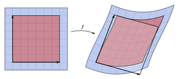
A nonlinear map  sends a small square (left, in red) to a distorted parallelogram (right, in red). The Jacobian at a point gives the best linear approximation of the distorted parallelogram near that point (right, in translucent white), and the Jacobian determinant gives the ratio of the area of the approximating parallelogram to that of the original square.
For a general differentiable function, much of the above carries over by considering the Jacobian matrix of f. For

the Jacobian matrix is the n × n matrix whose entries are given by the partial derivatives

Its determinant, the Jacobian determinant, appears in the higher-dimensional version of integration by substitution: for suitable functions f and an open subset U of Rn (the domain of f), the integral over f(U) of some other function φ : Rn → Rm is given by

The Jacobian also occurs in the inverse function theorem.
When applied to the field of Cartography, the determinant can be used to measure the rate of expansion of a map near the poles. [42]
Abstract algebraic aspects [edit]
Determinant of an endomorphism[edit]
The above identities concerning the determinant of products and inverses of matrices imply that similar matrices have the same determinant: two matrices A and B are similar, if there exists an invertible matrix X such that A = X−1BX. Indeed, repeatedly applying the above identities yields

The determinant is therefore also called a similarity invariant. The determinant of a linear transformation
for some finite-dimensional vector space V is defined to be the determinant of the matrix describing it, with respect to an arbitrary choice of basis in V. By the similarity invariance, this determinant is independent of the choice of the basis for V and therefore only depends on the endomorphism T.
Square matrices over commutative rings[edit]
The above definition of the determinant using the Leibniz rule holds works more generally when the entries of the matrix are elements of a commutative ring  , such as the integers
  , as opposed to the field of real or complex numbers. Moreover, the characterization of the determinant as the unique alternating multilinear map that satisfies
  still holds, as do all the properties that result from that characterization.[43]
A matrix  is invertible (in the sense that there is an inverse matrix whose entries are in ) if and only if its determinant is an invertible element in .[44] For
  , this means that the determinant is +1 or −1. Such a matrix is called unimodular.
The determinant being multiplicative, it defines a group homomorphism

between the general linear group (the group of invertible -matrices with entries in ) and the multiplicative group of units in . Since it respects the multiplication in both groups, this map is a group homomorphism.
![]()
The determinant is a natural transformation.
Given a ring homomorphism  , there is a map
  given by replacing all entries in by their images under
  . The determinant respects these maps, i.e., the identity

holds. In other words, the displayed commutative diagram commutes.
For example, the determinant of the complex conjugate of a complex matrix (which is also the determinant of its conjugate transpose) is the complex conjugate of its determinant, and for integer matrices: the reduction modulo  of the determinant of such a matrix is equal to the determinant of the matrix reduced modulo (the latter determinant being computed using modular arithmetic). In the language of category theory, the determinant is a natural transformation between the two functors and
  .[45] Adding yet another layer of abstraction, this is captured by saying that the determinant is a morphism of algebraic groups, from the general linear group to the multiplicative group,

Exterior algebra[edit]
The determinant of a linear transformation  of an -dimensional vector space
  or, more generally a free module of (finite) rank over a commutative ring can be formulated in a coordinate-free manner by considering the -th exterior power
  of .[46] The map
  induces a linear map

As is one-dimensional, the map  is given by multiplying with some scalar, i.e., an element in . Some authors such as (Bourbaki 1998) use this fact to define the determinant to be the element in satisfying the following identity (for all
  ):
):

This definition agrees with the more concrete coordinate-dependent definition. This can be shown using the uniqueness of a multilinear alternating form on -tuples of vectors in  .
.
For this reason, the highest non-zero exterior power (as opposed to the determinant associated to an endomorphism) is sometimes also called the determinant of and similarly for more involved objects such as vector bundles or chain complexes of vector spaces. Minors of a matrix can also be cast in this setting, by considering lower alternating forms  with
with  .[47]
.[47]
Generalizations and related notions[edit]
Determinants as treated above admit several variants: the permanent of a matrix is defined as the determinant, except that the factors occurring in Leibniz’s rule are omitted. The immanant generalizes both by introducing a character of the symmetric group in Leibniz’s rule.
Determinants for finite-dimensional algebras[edit]
For any associative algebra that is finite-dimensional as a vector space over a field  , there is a determinant map
[48]

This definition proceeds by establishing the characteristic polynomial independently of the determinant, and defining the determinant as the lowest order term of this polynomial. This general definition recovers the determinant for the matrix algebra  , but also includes several further cases including the determinant of a quaternion,
- ,

the norm  of a field extension, as well as the Pfaffian of a skew-symmetric matrix and the reduced norm of a central simple algebra, also arise as special cases of this construction.
Infinite matrices[edit]
For matrices with an infinite number of rows and columns, the above definitions of the determinant do not carry over directly. For example, in the Leibniz formula, an infinite sum (all of whose terms are infinite products) would have to be calculated. Functional analysis provides different extensions of the determinant for such infinite-dimensional situations, which however only work for particular kinds of operators.
The Fredholm determinant defines the determinant for operators known as trace class operators by an appropriate generalization of the formula

Another infinite-dimensional notion of determinant is the functional determinant.
Operators in von Neumann algebras[edit]
For operators in a finite factor, one may define a positive real-valued determinant called the Fuglede−Kadison determinant using the canonical trace. In fact, corresponding to every tracial state on a von Neumann algebra there is a notion of Fuglede−Kadison determinant.
[edit]
For matrices over non-commutative rings, multilinearity and alternating properties are incompatible for n ≥ 2,[49] so there is no good definition of the determinant in this setting.
For square matrices with entries in a non-commutative ring, there are various difficulties in defining determinants analogously to that for commutative rings. A meaning can be given to the Leibniz formula provided that the order for the product is specified, and similarly for other definitions of the determinant, but non-commutativity then leads to the loss of many fundamental properties of the determinant, such as the multiplicative property or that the determinant is unchanged under transposition of the matrix. Over non-commutative rings, there is no reasonable notion of a multilinear form (existence of a nonzero bilinear form[clarify] with a regular element of R as value on some pair of arguments implies that R is commutative). Nevertheless, various notions of non-commutative determinant have been formulated that preserve some of the properties of determinants, notably quasideterminants and the Dieudonné determinant. For some classes of matrices with non-commutative elements, one can define the determinant and prove linear algebra theorems that are very similar to their commutative analogs. Examples include the q-determinant on quantum groups, the Capelli determinant on Capelli matrices, and the Berezinian on supermatrices (i.e., matrices whose entries are elements of  -graded rings).[50] Manin matrices form the class closest to matrices with commutative elements.
Calculation[edit]
Determinants are mainly used as a theoretical tool. They are rarely calculated explicitly in numerical linear algebra, where for applications like checking invertibility and finding eigenvalues the determinant has largely been supplanted by other techniques.[51] Computational geometry, however, does frequently use calculations related to determinants.[52]
While the determinant can be computed directly using the Leibniz rule this approach is extremely inefficient for large matrices, since that formula requires calculating  ( factorial) products for an -matrix. Thus, the number of required operations grows very quickly: it is of order . The Laplace expansion is similarly inefficient. Therefore, more involved techniques have been developed for calculating determinants.
Decomposition methods[edit]
Some methods compute by writing the matrix as a product of matrices whose determinants can be more easily computed. Such techniques are referred to as decomposition methods. Examples include the LU decomposition, the QR decomposition or the Cholesky decomposition (for positive definite matrices). These methods are of order , which is a significant improvement over  .[53]
.[53]
For example, LU decomposition expresses as a product

of a permutation matrix  (which has exactly a single in each column, and otherwise zeros), a lower triangular matrix
  and an upper triangular matrix
  .
.
The determinants of the two triangular matrices and can be quickly calculated, since they are the products of the respective diagonal entries. The determinant of is just the sign  of the corresponding permutation (which is
  for an even number of permutations and is
  for an odd number of permutations). Once such a LU decomposition is known for , its determinant is readily computed as

Further methods[edit]
The order reached by decomposition methods has been improved by different methods. If two matrices of order can be multiplied in time  , where
  for some
  , then there is an algorithm computing the determinant in time
  .[54] This means, for example, that an
  algorithm for computing the determinant exists based on the Coppersmith–Winograd algorithm. This exponent has been further lowered, as of 2016, to 2.373.[55]
In addition to the complexity of the algorithm, further criteria can be used to compare algorithms.
Especially for applications concerning matrices over rings, algorithms that compute the determinant without any divisions exist. (By contrast, Gauss elimination requires divisions.) One such algorithm, having complexity  is based on the following idea: one replaces permutations (as in the Leibniz rule) by so-called closed ordered walks, in which several items can be repeated. The resulting sum has more terms than in the Leibniz rule, but in the process several of these products can be reused, making it more efficient than naively computing with the Leibniz rule.[56] Algorithms can also be assessed according to their bit complexity, i.e., how many bits of accuracy are needed to store intermediate values occurring in the computation. For example, the Gaussian elimination (or LU decomposition) method is of order , but the bit length of intermediate values can become exponentially long.[57] By comparison, the Bareiss Algorithm, is an exact-division method (so it does use division, but only in cases where these divisions can be performed without remainder) is of the same order, but the bit complexity is roughly the bit size of the original entries in the matrix times .[58]
If the determinant of A and the inverse of A have already been computed, the matrix determinant lemma allows rapid calculation of the determinant of A + uvT, where u and v are column vectors.
Charles Dodgson (i.e. Lewis Carroll of Alice’s Adventures in Wonderland fame) invented a method for computing determinants called Dodgson condensation. Unfortunately this interesting method does not always work in its original form.[59]
See also[edit]
- Cauchy determinant
- Cayley–Menger determinant
- Dieudonné determinant
- Slater determinant
- Determinantal conjecture
Notes[edit]
- ^ Lang 1985, §VII.1
- ^ Wildberger, Norman J. (2010). Episode 4 (video lecture). WildLinAlg. Sydney, Australia: University of New South Wales. Archived from the original on 2021-12-11 – via YouTube.
- ^ «Determinants and Volumes». textbooks.math.gatech.edu. Retrieved 16 March 2018.
- ^ McConnell (1957). Applications of Tensor Analysis. Dover Publications. pp. 10–17.
- ^ Harris 2014, §4.7
- ^ Serge Lang, Linear Algebra, 2nd Edition, Addison-Wesley, 1971, pp 173, 191.
- ^ Lang 1987, §VI.7, Theorem 7.5
- ^ Alternatively, Bourbaki 1998, §III.8, Proposition 1 proves this result using the functoriality of the exterior power.
- ^ Horn & Johnson 2018, §0.8.7
- ^ Kung, Rota & Yan 2009, p. 306
- ^ Horn & Johnson 2018, §0.8.2.
- ^
- ^ Silvester, J. R. (2000). «Determinants of Block Matrices». Math. Gazette. 84 (501): 460–467. doi:10.2307/3620776. JSTOR 3620776. S2CID 41879675.
- ^ Sothanaphan, Nat (January 2017). «Determinants of block matrices with noncommuting blocks». Linear Algebra and Its Applications. 512: 202–218. arXiv:1805.06027. doi:10.1016/j.laa.2016.10.004. S2CID 119272194.
- ^ Proofs can be found in http://www.ee.ic.ac.uk/hp/staff/dmb/matrix/proof003.html
- ^ Lin, Minghua; Sra, Suvrit (2014). «Completely strong superadditivity of generalized matrix functions». arXiv:1410.1958 [math.FA].
- ^ Paksoy; Turkmen; Zhang (2014). «Inequalities of Generalized Matrix Functions via Tensor Products». Electronic Journal of Linear Algebra. 27: 332–341. doi:10.13001/1081-3810.1622.
- ^ Serre, Denis (Oct 18, 2010). «Concavity of det1⁄n over HPDn«. MathOverflow.
- ^ Lang 1985, §VIII.2, Horn & Johnson 2018, Def. 1.2.3
- ^ Horn & Johnson 2018, Observation 7.1.2, Theorem 7.2.5
- ^ A proof can be found in the Appendix B of Kondratyuk, L. A.; Krivoruchenko, M. I. (1992). «Superconducting quark matter in SU(2) color group». Zeitschrift für Physik A. 344 (1): 99–115. Bibcode:1992ZPhyA.344…99K. doi:10.1007/BF01291027. S2CID 120467300.
- ^ Horn & Johnson 2018, § 0.8.10
- ^ Grattan-Guinness 2003, §6.6
- ^ Cajori, F. A History of Mathematics p. 80
- ^ a b c Campbell, H: «Linear Algebra With Applications», pages 111–112. Appleton Century Crofts, 1971
- ^ Eves 1990, p. 405
- ^ A Brief History of Linear Algebra and Matrix Theory at: «A Brief History of Linear Algebra and Matrix Theory». Archived from the original on 10 September 2012. Retrieved 24 January 2012.
- ^ Kleiner 2004, p. 80
- ^ Bourbaki (1994, p. 59)
- ^ Muir, Sir Thomas, The Theory of Determinants in the historical Order of Development [London, England: Macmillan and Co., Ltd., 1906]. JFM 37.0181.02
- ^ Kleiner 2007, §5.2
- ^ The first use of the word «determinant» in the modern sense appeared in: Cauchy, Augustin-Louis «Memoire sur les fonctions qui ne peuvent obtenir que deux valeurs égales et des signes contraires par suite des transpositions operées entre les variables qu’elles renferment,» which was first read at the Institute de France in Paris on November 30, 1812, and which was subsequently published in the Journal de l’Ecole Polytechnique, Cahier 17, Tome 10, pages 29–112 (1815).
- ^ Origins of mathematical terms: http://jeff560.tripod.com/d.html
- ^ History of matrices and determinants: http://www-history.mcs.st-and.ac.uk/history/HistTopics/Matrices_and_determinants.html
- ^ Eves 1990, p. 494
- ^ Cajori 1993, Vol. II, p. 92, no. 462
- ^ History of matrix notation: http://jeff560.tripod.com/matrices.html
- ^ Habgood & Arel 2012
- ^ Lang 1985, §VII.3
- ^ Lang 2002, §IV.8
- ^ Lang 1985, §VII.6, Theorem 6.10
- ^ Lay, David (2021). Linear Algebra and It’s Applications 6th Edition. Pearson. p. 172.
- ^ Dummit & Foote 2004, §11.4
- ^ Dummit & Foote 2004, §11.4, Theorem 30
- ^ Mac Lane 1998, §I.4. See also Natural transformation § Determinant.
- ^ Bourbaki 1998, §III.8
- ^ Lombardi & Quitté 2015, §5.2, Bourbaki 1998, §III.5
- ^ Garibaldi 2004
- ^ In a non-commutative setting left-linearity (compatibility with left-multiplication by scalars) should be distinguished from right-linearity. Assuming linearity in the columns is taken to be left-linearity, one would have, for non-commuting scalars a, b:
a contradiction. There is no useful notion of multi-linear functions over a non-commutative ring.
- ^ Varadarajan, V. S (2004), Supersymmetry for mathematicians: An introduction, ISBN 978-0-8218-3574-6.
- ^ «… we mention that the determinant, though a convenient notion theoretically, rarely finds a useful role in numerical algorithms.», see Trefethen & Bau III 1997, Lecture 1.
- ^ Fisikopoulos & Peñaranda 2016, §1.1, §4.3
- ^ Camarero, Cristóbal (2018-12-05). «Simple, Fast and Practicable Algorithms for Cholesky, LU and QR Decomposition Using Fast Rectangular Matrix Multiplication». arXiv:1812.02056 [cs.NA].
- ^ Bunch & Hopcroft 1974
- ^ Fisikopoulos & Peñaranda 2016, §1.1
- ^ Rote 2001
- ^ Fang, Xin Gui; Havas, George (1997). «On the worst-case complexity of integer Gaussian elimination» (PDF). Proceedings of the 1997 international symposium on Symbolic and algebraic computation. ISSAC ’97. Kihei, Maui, Hawaii, United States: ACM. pp. 28–31. doi:10.1145/258726.258740. ISBN 0-89791-875-4. Archived from the original (PDF) on 2011-08-07. Retrieved 2011-01-22.
- ^ Fisikopoulos & Peñaranda 2016, §1.1, Bareiss 1968
- ^ Abeles, Francine F. (2008). «Dodgson condensation: The historical and mathematical development of an experimental method». Linear Algebra and Its Applications. 429 (2–3): 429–438. doi:10.1016/j.laa.2007.11.022.


References[edit]
- Anton, Howard (2005), Elementary Linear Algebra (Applications Version) (9th ed.), Wiley International
- Axler, Sheldon Jay (2015). Linear Algebra Done Right (3rd ed.). Springer. ISBN 978-3-319-11079-0.
- Bareiss, Erwin (1968), «Sylvester’s Identity and Multistep Integer-Preserving Gaussian Elimination» (PDF), Mathematics of Computation, 22 (102): 565–578, doi:10.2307/2004533, JSTOR 2004533, archived (PDF) from the original on 2012-10-25
- de Boor, Carl (1990), «An empty exercise» (PDF), ACM SIGNUM Newsletter, 25 (2): 3–7, doi:10.1145/122272.122273, S2CID 62780452, archived (PDF) from the original on 2006-09-01
- Bourbaki, Nicolas (1998), Algebra I, Chapters 1-3, Springer, ISBN 9783540642435
- Bunch, J. R.; Hopcroft, J. E. (1974). «Triangular Factorization and Inversion by Fast Matrix Multiplication». Mathematics of Computation. 28 (125): 231–236. doi:10.1090/S0025-5718-1974-0331751-8.
- Dummit, David S.; Foote, Richard M. (2004), Abstract algebra (3rd ed.), Hoboken, NJ: Wiley, ISBN 9780471452348, OCLC 248917264
- Fisikopoulos, Vissarion; Peñaranda, Luis (2016), «Faster geometric algorithms via dynamic determinant computation», Computational Geometry, 54: 1–16, doi:10.1016/j.comgeo.2015.12.001
- Garibaldi, Skip (2004), «The characteristic polynomial and determinant are not ad hoc constructions», American Mathematical Monthly, 111 (9): 761–778, arXiv:math/0203276, doi:10.2307/4145188, JSTOR 4145188, MR 2104048
- Habgood, Ken; Arel, Itamar (2012). «A condensation-based application of Cramer’s rule for solving large-scale linear systems» (PDF). Journal of Discrete Algorithms. 10: 98–109. doi:10.1016/j.jda.2011.06.007. Archived (PDF) from the original on 2019-05-05.
- Harris, Frank E. (2014), Mathematics for Physical Science and Engineering, Elsevier, ISBN 9780128010495
- Kleiner, Israel (2007), Kleiner, Israel (ed.), A history of abstract algebra, Birkhäuser, doi:10.1007/978-0-8176-4685-1, ISBN 978-0-8176-4684-4, MR 2347309
- Kung, Joseph P.S.; Rota, Gian-Carlo; Yan, Catherine (2009), Combinatorics: The Rota Way, Cambridge University Press, ISBN 9780521883894
- Lay, David C. (August 22, 2005), Linear Algebra and Its Applications (3rd ed.), Addison Wesley, ISBN 978-0-321-28713-7
- Lombardi, Henri; Quitté, Claude (2015), Commutative Algebra: Constructive Methods, Springer, ISBN 9789401799447
- Mac Lane, Saunders (1998), Categories for the Working Mathematician, Graduate Texts in Mathematics 5 (2nd ed.), Springer-Verlag, ISBN 0-387-98403-8
- Meyer, Carl D. (February 15, 2001), Matrix Analysis and Applied Linear Algebra, Society for Industrial and Applied Mathematics (SIAM), ISBN 978-0-89871-454-8, archived from the original on 2009-10-31
- Muir, Thomas (1960) [1933], A treatise on the theory of determinants, Revised and enlarged by William H. Metzler, New York, NY: Dover
- Poole, David (2006), Linear Algebra: A Modern Introduction (2nd ed.), Brooks/Cole, ISBN 0-534-99845-3
- G. Baley Price (1947) «Some identities in the theory of determinants», American Mathematical Monthly 54:75–90 MR0019078
- Horn, Roger Alan; Johnson, Charles Royal (2018) [1985]. Matrix Analysis (2nd ed.). Cambridge University Press. ISBN 978-0-521-54823-6.
- Lang, Serge (1985), Introduction to Linear Algebra, Undergraduate Texts in Mathematics (2 ed.), Springer, ISBN 9780387962054
- Lang, Serge (1987), Linear Algebra, Undergraduate Texts in Mathematics (3 ed.), Springer, ISBN 9780387964126
- Lang, Serge (2002). Algebra. Graduate Texts in Mathematics. New York, NY: Springer. ISBN 978-0-387-95385-4.
- Leon, Steven J. (2006), Linear Algebra With Applications (7th ed.), Pearson Prentice Hall
- Rote, Günter (2001), «Division-free algorithms for the determinant and the Pfaffian: algebraic and combinatorial approaches» (PDF), Computational discrete mathematics, Lecture Notes in Comput. Sci., vol. 2122, Springer, pp. 119–135, doi:10.1007/3-540-45506-X_9, ISBN 978-3-540-42775-9, MR 1911585, archived from the original (PDF) on 2007-02-01, retrieved 2020-06-04
- Trefethen, Lloyd; Bau III, David (1997), Numerical Linear Algebra (1st ed.), Philadelphia: SIAM, ISBN 978-0-89871-361-9
Historical references[edit]
- Bourbaki, Nicolas (1994), Elements of the history of mathematics, translated by Meldrum, John, Springer, doi:10.1007/978-3-642-61693-8, ISBN 3-540-19376-6
- Cajori, Florian (1993), A history of mathematical notations: Including Vol. I. Notations in elementary mathematics; Vol. II. Notations mainly in higher mathematics, Reprint of the 1928 and 1929 originals, Dover, ISBN 0-486-67766-4, MR 3363427
- Bezout, Étienne (1779), Théorie générale des equations algébriques, Paris
- Cayley, Arthur (1841), «On a theorem in the geometry of position», Cambridge Mathematical Journal, 2: 267–271
- Cramer, Gabriel (1750), Introduction à l’analyse des lignes courbes algébriques, Genève: Frères Cramer & Cl. Philibert, doi:10.3931/e-rara-4048
- Eves, Howard (1990), An introduction to the history of mathematics (6 ed.), Saunders College Publishing, ISBN 0-03-029558-0, MR 1104435
- Grattan-Guinness, I., ed. (2003), Companion Encyclopedia of the History and Philosophy of the Mathematical Sciences, vol. 1, Johns Hopkins University Press, ISBN 9780801873966
- Jacobi, Carl Gustav Jakob (1841), «De Determinantibus functionalibus», Journal für die reine und angewandte Mathematik, 1841 (22): 320–359, doi:10.1515/crll.1841.22.319, S2CID 123637858
- Laplace, Pierre-Simon, de (1772), «Recherches sur le calcul intégral et sur le systéme du monde», Histoire de l’Académie Royale des Sciences, Paris (seconde partie): 267–376
External links[edit]
![]()
- Suprunenko, D.A. (2001) [1994], «Determinant», Encyclopedia of Mathematics, EMS Press
- Weisstein, Eric W. «Determinant». MathWorld.
- O’Connor, John J.; Robertson, Edmund F., «Matrices and determinants», MacTutor History of Mathematics archive, University of St Andrews
- Determinant Interactive Program and Tutorial
- Linear algebra: determinants. Archived 2008-12-04 at the Wayback Machine Compute determinants of matrices up to order 6 using Laplace expansion you choose.
- Determinant Calculator Calculator for matrix determinants, up to the 8th order.
- Matrices and Linear Algebra on the Earliest Uses Pages
- Determinants explained in an easy fashion in the 4th chapter as a part of a Linear Algebra course.
This article is about mathematics. For determinants in epidemiology, see Risk factor. For determinants in immunology, see Epitope.
In mathematics, the determinant is a scalar value that is a function of the entries of a square matrix. It characterizes some properties of the matrix and the linear map represented by the matrix. In particular, the determinant is nonzero if and only if the matrix is invertible and the linear map represented by the matrix is an isomorphism. The determinant of a product of matrices is the product of their determinants (the preceding property is a corollary of this one).
The determinant of a matrix A is denoted det(A), det A, or |A|.
The determinant of a 2 × 2 matrix is
and the determinant of a 3 × 3 matrix is
The determinant of a n × n matrix can be defined in several equivalent ways. Leibniz formula expresses the determinant as a sum of signed products of matrix entries such that each summand is the product of n different entries, and the number of these summands is the factorial of n (the product of the n first positive integers). The Laplace expansion expresses the determinant of a n × n matrix as a linear combination of determinants of submatrices. Gaussian elimination express the determinant as the product of the diagonal entries of a diagonal matrix that is obtained by a succession of elementary row operations.
Determinants can also be defined by some of their properties: the determinant is the unique function defined on the n × n matrices that has the four following properties. The determinant of the identity matrix is 1; the exchange of two rows (or of two columns) multiplies the determinant by −1; multiplying a row (or a column) by a number multiplies the determinant by this number; and adding to a row (or a column) a multiple of another row (or column) does not change the determinant.
Determinants occur throughout mathematics. For example, a matrix is often used to represent the coefficients in a system of linear equations, and determinants can be used to solve these equations (Cramer’s rule), although other methods of solution are computationally much more efficient. Determinants are used for defining the characteristic polynomial of a matrix, whose roots are the eigenvalues. In geometry, the signed n-dimensional volume of a n-dimensional parallelepiped is expressed by a determinant. This is used in calculus with exterior differential forms and the Jacobian determinant, in particular for changes of variables in multiple integrals.
2 × 2 matrices[edit]
The determinant of a 2 × 2 matrix is denoted either by «det» or by vertical bars around the matrix, and is defined as
For example,
First properties[edit]
The determinant has several key properties that can be proved by direct evaluation of the definition for -matrices, and that continue to hold for determinants of larger matrices. They are as follows:[1] first, the determinant of the identity matrix is 1.
Second, the determinant is zero if two rows are the same:
This holds similarly if the two columns are the same. Moreover,
Finally, if any column is multiplied by some number (i.e., all entries in that column are multiplied by that number), the determinant is also multiplied by that number:
Geometric meaning[edit]
The area of the parallelogram is the absolute value of the determinant of the matrix formed by the vectors representing the parallelogram’s sides.
If the matrix entries are real numbers, the matrix A can be used to represent two linear maps: one that maps the standard basis vectors to the rows of A, and one that maps them to the columns of A. In either case, the images of the basis vectors form a parallelogram that represents the image of the unit square under the mapping. The parallelogram defined by the rows of the above matrix is the one with vertices at (0, 0), (a, b), (a + c, b + d), and (c, d), as shown in the accompanying diagram.
The absolute value of ad − bc is the area of the parallelogram, and thus represents the scale factor by which areas are transformed by A. (The parallelogram formed by the columns of A is in general a different parallelogram, but since the determinant is symmetric with respect to rows and columns, the area will be the same.)
The absolute value of the determinant together with the sign becomes the oriented area of the parallelogram. The oriented area is the same as the usual area, except that it is negative when the angle from the first to the second vector defining the parallelogram turns in a clockwise direction (which is opposite to the direction one would get for the identity matrix).
To show that ad − bc is the signed area, one may consider a matrix containing two vectors u ≡ (a, b) and v ≡ (c, d) representing the parallelogram’s sides. The signed area can be expressed as |u| |v| sin θ for the angle θ between the vectors, which is simply base times height, the length of one vector times the perpendicular component of the other. Due to the sine this already is the signed area, yet it may be expressed more conveniently using the cosine of the complementary angle to a perpendicular vector, e.g. u⊥ = (−b, a), so that |u⊥| |v| cos θ′, which can be determined by the pattern of the scalar product to be equal to ad − bc:
The volume of this parallelepiped is the absolute value of the determinant of the matrix formed by the columns constructed from the vectors r1, r2, and r3.
Thus the determinant gives the scaling factor and the orientation induced by the mapping represented by A. When the determinant is equal to one, the linear mapping defined by the matrix is equi-areal and orientation-preserving.
The object known as the bivector is related to these ideas. In 2D, it can be interpreted as an oriented plane segment formed by imagining two vectors each with origin (0, 0), and coordinates (a, b) and (c, d). The bivector magnitude (denoted by (a, b) ∧ (c, d)) is the signed area, which is also the determinant ad − bc.[2]
If an n × n real matrix A is written in terms of its column vectors , then
This means that maps the unit n-cube to the n-dimensional parallelotope defined by the vectors the region
The determinant gives the signed n-dimensional volume of this parallelotope, and hence describes more generally the n-dimensional volume scaling factor of the linear transformation produced by A.[3] (The sign shows whether the transformation preserves or reverses orientation.) In particular, if the determinant is zero, then this parallelotope has volume zero and is not fully n-dimensional, which indicates that the dimension of the image of A is less than n. This means that A produces a linear transformation which is neither onto nor one-to-one, and so is not invertible.
Definition[edit]
In the sequel, A is a square matrix with n rows and n columns, so that it can be written as
The entries etc. are, for many purposes, real or complex numbers. As discussed below, the determinant is also defined for matrices whose entries are in a commutative ring.
The determinant of A is denoted by det(A), or it can be denoted directly in terms of the matrix entries by writing enclosing bars instead of brackets:
There are various equivalent ways to define the determinant of a square matrix A, i.e. one with the same number of rows and columns: the determinant can be defined via the Leibniz formula, an explicit formula involving sums of products of certain entries of the matrix. The determinant can also be characterized as the unique function depending on the entries of the matrix satisfying certain properties. This approach can also be used to compute determinants by simplifying the matrices in question.
Leibniz formula[edit]
3 × 3 matrices[edit]
The Leibniz formula for the determinant of a 3 × 3 matrix is the following:
The rule of Sarrus is a mnemonic for the expanded form of this determinant: the sum of the products of three diagonal north-west to south-east lines of matrix elements, minus the sum of the products of three diagonal south-west to north-east lines of elements, when the copies of the first two columns of the matrix are written beside it as in the illustration. This scheme for calculating the determinant of a 3 × 3 matrix does not carry over into higher dimensions.
n × n matrices[edit]
In higher dimension, the Leibniz formula expresses the determinant of an -matrix as an expression involving permutations and their signatures. A permutation of the set is a function that reorders this set of integers. The value in the -th position after the reordering is denoted below by . The set of all such permutations, called the symmetric group, is commonly denoted . The signature of a permutation is if the permutation can be obtained with an even number of exchanges of two entries; otherwise, it is
Given a matrix
the Leibniz formula for its determinant is, using sigma notation,
Using pi notation, this can be shortened into
- .
The Levi-Civita symbol is defined on the n-tuples of integers in as 0 if two of the integers are equal, and, otherwise, as the signature of the permutation defined by the tuple of integers. With the Levi-Civita symbol, Leibniz formula may be written as
where the sum is taken over all n-tuples of integers in
[4][5]
Properties of the determinant[edit]
Characterization of the determinant[edit]
The determinant can be characterized by the following three key properties. To state these, it is convenient to regard an -matrix A as being composed of its columns, so denoted as
where the column vector (for each i) is composed of the entries of the matrix in the i-th column.
- , where is an identity matrix.
- The determinant is multilinear: if the jth column of a matrix is written as a linear combination of two column vectors v and w and a number r, then the determinant of A is expressible as a similar linear combination:
- The determinant is alternating: whenever two columns of a matrix are identical, its determinant is 0:
If the determinant is defined using the Leibniz formula as above, these three properties can be proved by direct inspection of that formula. Some authors also approach the determinant directly using these three properties: it can be shown that there is exactly one function that assigns to any -matrix A a number that satisfies these three properties.[6] This also shows that this more abstract approach to the determinant yields the same definition as the one using the Leibniz formula.
To see this it suffices to expand the determinant by multi-linearity in the columns into a (huge) linear combination of determinants of matrices in which each column is a standard basis vector. These determinants are either 0 (by property 9) or else ±1 (by properties 1 and 12 below), so the linear combination gives the expression above in terms of the Levi-Civita symbol. While less technical in appearance, this characterization cannot entirely replace the Leibniz formula in defining the determinant, since without it the existence of an appropriate function is not clear.[citation needed]
Immediate consequences[edit]
These rules have several further consequences:
- The determinant is a homogeneous function, i.e.,
(for an
matrix ). - Interchanging any pair of columns of a matrix multiplies its determinant by −1. This follows from the determinant being multilinear and alternating (properties 2 and 3 above):
This formula can be applied iteratively when several columns are swapped. For example
Yet more generally, any permutation of the columns multiplies the determinant by the sign of the permutation.
- If some column can be expressed as a linear combination of the other columns (i.e. the columns of the matrix form a linearly dependent set), the determinant is 0. As a special case, this includes: if some column is such that all its entries are zero, then the determinant of that matrix is 0.
- Adding a scalar multiple of one column to another column does not change the value of the determinant. This is a consequence of multilinearity and being alternative: by multilinearity the determinant changes by a multiple of the determinant of a matrix with two equal columns, which determinant is 0, since the determinant is alternating.
- If is a triangular matrix, i.e. , whenever or, alternatively, whenever , then its determinant equals the product of the diagonal entries:
Indeed, such a matrix can be reduced, by appropriately adding multiples of the columns with fewer nonzero entries to those with more entries, to a diagonal matrix (without changing the determinant). For such a matrix, using the linearity in each column reduces to the identity matrix, in which case the stated formula holds by the very first characterizing property of determinants. Alternatively, this formula can also be deduced from the Leibniz formula, since the only permutation
which gives a non-zero contribution is the identity permutation.
Example[edit]
These characterizing properties and their consequences listed above are both theoretically significant, but can also be used to compute determinants for concrete matrices. In fact, Gaussian elimination can be applied to bring any matrix into upper triangular form, and the steps in this algorithm affect the determinant in a controlled way. The following concrete example illustrates the computation of the determinant of the matrix using that method:
| Matrix | |
|
|
|
| Obtained by |
add the second column to the first |
add 3 times the third column to the second |
swap the first two columns |
add |
| Determinant | |
|
|
|
Combining these equalities gives
Transpose[edit]
The determinant of the transpose of equals the determinant of A:
- .
This can be proven by inspecting the Leibniz formula.[7] This implies that in all the properties mentioned above, the word «column» can be replaced by «row» throughout. For example, viewing an n × n matrix as being composed of n rows, the determinant is an n-linear function.
Multiplicativity and matrix groups[edit]
The determinant is a multiplicative map, i.e., for square matrices and of equal size, the determinant of a matrix product equals the product of their determinants:
This key fact can be proven by observing that, for a fixed matrix , both sides of the equation are alternating and multilinear as a function depending on the columns of . Moreover, they both take the value when is the identity matrix. The above-mentioned unique characterization of alternating multilinear maps therefore shows this claim.[8]
A matrix is invertible precisely if its determinant is nonzero. This follows from the multiplicativity of and the formula for the inverse involving the adjugate matrix mentioned below. In this event, the determinant of the inverse matrix is given by
- .
In particular, products and inverses of matrices with non-zero determinant (respectively, determinant one) still have this property. Thus, the set of such matrices (of fixed size ) forms a group known as the general linear group (respectively, a subgroup called the special linear group . More generally, the word «special» indicates the subgroup of another matrix group of matrices of determinant one. Examples include the special orthogonal group (which if n is 2 or 3 consists of all rotation matrices), and the special unitary group.
The Cauchy–Binet formula is a generalization of that product formula for rectangular matrices. This formula can also be recast as a multiplicative formula for compound matrices whose entries are the determinants of all quadratic submatrices of a given matrix.[9][10]
Laplace expansion[edit]
Laplace expansion expresses the determinant of a matrix in terms of determinants of smaller matrices, known as its minors. The minor is defined to be the determinant of the -matrix that results from by removing the -th row and the -th column. The expression is known as a cofactor. For every , one has the equality
which is called the Laplace expansion along the ith row. For example, the Laplace expansion along the first row () gives the following formula:
Unwinding the determinants of these -matrices gives back the Leibniz formula mentioned above. Similarly, the Laplace expansion along the -th column is the equality
Laplace expansion can be used iteratively for computing determinants, but this approach is inefficient for large matrices. However, it is useful for computing the determinants of highly symmetric matrix such as the Vandermonde matrix
This determinant has been applied, for example, in the proof of Baker’s theorem in the theory of transcendental numbers.
Adjugate matrix[edit]
The adjugate matrix is the transpose of the matrix of the cofactors, that is,
For every matrix, one has[11]
Thus the adjugate matrix can be used for expressing the inverse of a nonsingular matrix:
Block matrices[edit]
The formula for the determinant of a -matrix above continues to hold, under appropriate further assumptions, for a block matrix, i.e., a matrix composed of four submatrices of dimension , , and , respectively. The easiest such formula, which can be proven using either the Leibniz formula or a factorization involving the Schur complement, is
If is invertible (and similarly if is invertible[12]), one has
If is a -matrix, this simplifies to .
If the blocks are square matrices of the same size further formulas hold. For example, if and commute (i.e., ), then there holds [13]
This formula has been generalized to matrices composed of more than blocks, again under appropriate commutativity conditions among the individual blocks.[14]
For and , the following formula holds (even if and do not commute)[citation needed]
Sylvester’s determinant theorem[edit]
Sylvester’s determinant theorem states that for A, an m × n matrix, and B, an n × m matrix (so that A and B have dimensions allowing them to be multiplied in either order forming a square matrix):
where Im and In are the m × m and n × n identity matrices, respectively.
From this general result several consequences follow.
Sum[edit]
The determinant of the sum of two square matrices of the same size is not in general expressible in terms of the determinants of A and of B. However, for positive semidefinite matrices , and of equal size,
with the corollary[16][17]
Conversely, if and are Hermitian, positive-definite, and size , then the determinant has concave th root;[18] this implies
by homogeneity.
Sum identity for 2×2 matrices[edit]
For the special case of matrices with complex entries, the determinant of the sum can be written in terms of determinants and traces in the following identity:
Proof of identity
This can be shown by writing out each term in components . The left-hand side is
Expanding gives
The terms which are quadratic in are seen to be , and similarly for , so the expression can be written
We can then write the cross-terms as
which can be recognized as
which completes the proof.
This has an application to matrix algebras. For example, consider the complex numbers as a matrix algebra. The complex numbers have a representation as matrices of the form
with and real. Since , taking and in the above identity gives
This result followed just from and .
Properties of the determinant in relation to other notions[edit]
Eigenvalues and characteristic polynomial[edit]
The determinant is closely related to two other central concepts in linear algebra, the eigenvalues and the characteristic polynomial of a matrix. Let be an -matrix with complex entries with eigenvalues . (Here it is understood that an eigenvalue with algebraic multiplicity μ occurs μ times in this list.) Then the determinant of A is the product of all eigenvalues,
The product of all non-zero eigenvalues is referred to as pseudo-determinant.
The characteristic polynomial is defined as[19]
Here, is the indeterminate of the polynomial and is the identity matrix of the same size as . By means of this polynomial, determinants can be used to find the eigenvalues of the matrix : they are precisely the roots of this polynomial, i.e., those complex numbers such that
A Hermitian matrix is positive definite if all its eigenvalues are positive. Sylvester’s criterion asserts that this is equivalent to the determinants of the submatrices
being positive, for all between and .[20]
Trace[edit]
The trace tr(A) is by definition the sum of the diagonal entries of A and also equals the sum of the eigenvalues. Thus, for complex matrices A,
or, for real matrices A,
Here exp(A) denotes the matrix exponential of A, because every eigenvalue λ of A corresponds to the eigenvalue exp(λ) of exp(A). In particular, given any logarithm of A, that is, any matrix L satisfying
the determinant of A is given by
For example, for n = 2, n = 3, and n = 4, respectively,
cf. Cayley-Hamilton theorem. Such expressions are deducible from combinatorial arguments, Newton’s identities, or the Faddeev–LeVerrier algorithm. That is, for generic n, detA = (−1)nc0 the signed constant term of the characteristic polynomial, determined recursively from
In the general case, this may also be obtained from[21]
where the sum is taken over the set of all integers kl ≥ 0 satisfying the equation
The formula can be expressed in terms of the complete exponential Bell polynomial of n arguments sl = −(l – 1)! tr(Al) as
This formula can also be used to find the determinant of a matrix AIJ with multidimensional indices I = (i1, i2, …, ir) and J = (j1, j2, …, jr). The product and trace of such matrices are defined in a natural way as
An important arbitrary dimension n identity can be obtained from the Mercator series expansion of the logarithm when the expansion converges. If every eigenvalue of A is less than 1 in absolute value,
where I is the identity matrix. More generally, if
is expanded as a formal power series in s then all coefficients of sm for m > n are zero and the remaining polynomial is det(I + sA).
Upper and lower bounds[edit]
For a positive definite matrix A, the trace operator gives the following tight lower and upper bounds on the log determinant
with equality if and only if A = I. This relationship can be derived via the formula for the Kullback-Leibler divergence between two multivariate normal distributions.
Also,
These inequalities can be proved by expressing the traces and the determinant in terms of the eigenvalues. As such, they represent the well-known fact that the harmonic mean is less than the geometric mean, which is less than the arithmetic mean, which is, in turn, less than the root mean square.
Derivative[edit]
The Leibniz formula shows that the determinant of real (or analogously for complex) square matrices is a polynomial function from to . In particular, it is everywhere differentiable. Its derivative can be expressed using Jacobi’s formula:[22]
where denotes the adjugate of . In particular, if is invertible, we have
Expressed in terms of the entries of , these are
Yet another equivalent formulation is
- ,
using big O notation. The special case where , the identity matrix, yields
This identity is used in describing Lie algebras associated to certain matrix Lie groups. For example, the special linear group is defined by the equation . The above formula shows that its Lie algebra is the special linear Lie algebra consisting of those matrices having trace zero.
Writing a -matrix as where are column vectors of length 3, then the gradient over one of the three vectors may be written as the cross product of the other two:
History[edit]
Historically, determinants were used long before matrices: A determinant was originally defined as a property of a system of linear equations.
The determinant «determines» whether the system has a unique solution (which occurs precisely if the determinant is non-zero).
In this sense, determinants were first used in the Chinese mathematics textbook The Nine Chapters on the Mathematical Art (九章算術, Chinese scholars, around the 3rd century BCE). In Europe, solutions of linear systems of two equations were expressed by Cardano in 1545 by a determinant-like entity.[23]
Determinants proper originated from the work of Seki Takakazu in 1683 in Japan and parallelly of Leibniz in 1693.[24][25][26][27] Cramer (1750) stated, without proof, Cramer’s rule.[28] Both Cramer and also Bezout (1779) were led to determinants by the question of plane curves passing through a given set of points.[29]
Vandermonde (1771) first recognized determinants as independent functions.[25] Laplace (1772) gave the general method of expanding a determinant in terms of its complementary minors: Vandermonde had already given a special case.[30] Immediately following, Lagrange (1773) treated determinants of the second and third order and applied it to questions of elimination theory; he proved many special cases of general identities.
Gauss (1801) made the next advance. Like Lagrange, he made much use of determinants in the theory of numbers. He introduced the word «determinant» (Laplace had used «resultant»), though not in the present signification, but rather as applied to the discriminant of a quantic.[31] Gauss also arrived at the notion of reciprocal (inverse) determinants, and came very near the multiplication theorem.
The next contributor of importance is Binet (1811, 1812), who formally stated the theorem relating to the product of two matrices of m columns and n rows, which for the special case of m = n reduces to the multiplication theorem. On the same day (November 30, 1812) that Binet presented his paper to the Academy, Cauchy also presented one on the subject. (See Cauchy–Binet formula.) In this he used the word «determinant» in its present sense,[32][33] summarized and simplified what was then known on the subject, improved the notation, and gave the multiplication theorem with a proof more satisfactory than Binet’s.[25][34] With him begins the theory in its generality.
(Jacobi 1841) used the functional determinant which Sylvester later called the Jacobian.[35] In his memoirs in Crelle’s Journal for 1841 he specially treats this subject, as well as the class of alternating functions which Sylvester has called alternants. About the time of Jacobi’s last memoirs, Sylvester (1839) and Cayley began their work. Cayley 1841 introduced the modern notation for the determinant using vertical bars.[36][37]
The study of special forms of determinants has been the natural result of the completion of the general theory. Axisymmetric determinants have been studied by Lebesgue, Hesse, and Sylvester; persymmetric determinants by Sylvester and Hankel; circulants by Catalan, Spottiswoode, Glaisher, and Scott; skew determinants and Pfaffians, in connection with the theory of orthogonal transformation, by Cayley; continuants by Sylvester; Wronskians (so called by Muir) by Christoffel and Frobenius; compound determinants by Sylvester, Reiss, and Picquet; Jacobians and Hessians by Sylvester; and symmetric gauche determinants by Trudi. Of the textbooks on the subject Spottiswoode’s was the first. In America, Hanus (1886), Weld (1893), and Muir/Metzler (1933) published treatises.
Applications[edit]
Cramer’s rule[edit]
Determinants can be used to describe the solutions of a linear system of equations, written in matrix form as . This equation has a unique solution if and only if is nonzero. In this case, the solution is given by Cramer’s rule:
where is the matrix formed by replacing the -th column of by the column vector . This follows immediately by column expansion of the determinant, i.e.
where the vectors are the columns of A. The rule is also implied by the identity
Cramer’s rule can be implemented in time, which is comparable to more common methods of solving systems of linear equations, such as LU, QR, or singular value decomposition.[38]
Linear independence[edit]
Determinants can be used to characterize linearly dependent vectors: is zero if and only if the column vectors (or, equivalently, the row vectors) of the matrix are linearly dependent.[39] For example, given two linearly independent vectors , a third vector lies in the plane spanned by the former two vectors exactly if the determinant of the -matrix consisting of the three vectors is zero. The same idea is also used in the theory of differential equations: given functions (supposed to be times differentiable), the Wronskian is defined to be
It is non-zero (for some ) in a specified interval if and only if the given functions and all their derivatives up to order are linearly independent. If it can be shown that the Wronskian is zero everywhere on an interval then, in the case of analytic functions, this implies the given functions are linearly dependent. See the Wronskian and linear independence. Another such use of the determinant is the resultant, which gives a criterion when two polynomials have a common root.[40]
Orientation of a basis[edit]
The determinant can be thought of as assigning a number to every sequence of n vectors in Rn, by using the square matrix whose columns are the given vectors. For instance, an orthogonal matrix with entries in Rn represents an orthonormal basis in Euclidean space. The determinant of such a matrix determines whether the orientation of the basis is consistent with or opposite to the orientation of the standard basis. If the determinant is +1, the basis has the same orientation. If it is −1, the basis has the opposite orientation.
More generally, if the determinant of A is positive, A represents an orientation-preserving linear transformation (if A is an orthogonal 2 × 2 or 3 × 3 matrix, this is a rotation), while if it is negative, A switches the orientation of the basis.
Volume and Jacobian determinant[edit]
As pointed out above, the absolute value of the determinant of real vectors is equal to the volume of the parallelepiped spanned by those vectors. As a consequence, if is the linear map given by multiplication with a matrix , and is any measurable subset, then the volume of is given by times the volume of .[41] More generally, if the linear map is represented by the -matrix , then the -dimensional volume of is given by:
By calculating the volume of the tetrahedron bounded by four points, they can be used to identify skew lines. The volume of any tetrahedron, given its vertices , , or any other combination of pairs of vertices that form a spanning tree over the vertices.
A nonlinear map sends a small square (left, in red) to a distorted parallelogram (right, in red). The Jacobian at a point gives the best linear approximation of the distorted parallelogram near that point (right, in translucent white), and the Jacobian determinant gives the ratio of the area of the approximating parallelogram to that of the original square.
For a general differentiable function, much of the above carries over by considering the Jacobian matrix of f. For
the Jacobian matrix is the n × n matrix whose entries are given by the partial derivatives
Its determinant, the Jacobian determinant, appears in the higher-dimensional version of integration by substitution: for suitable functions f and an open subset U of Rn (the domain of f), the integral over f(U) of some other function φ : Rn → Rm is given by
The Jacobian also occurs in the inverse function theorem.
When applied to the field of Cartography, the determinant can be used to measure the rate of expansion of a map near the poles. [42]
Abstract algebraic aspects [edit]
Determinant of an endomorphism[edit]
The above identities concerning the determinant of products and inverses of matrices imply that similar matrices have the same determinant: two matrices A and B are similar, if there exists an invertible matrix X such that A = X−1BX. Indeed, repeatedly applying the above identities yields
The determinant is therefore also called a similarity invariant. The determinant of a linear transformation
for some finite-dimensional vector space V is defined to be the determinant of the matrix describing it, with respect to an arbitrary choice of basis in V. By the similarity invariance, this determinant is independent of the choice of the basis for V and therefore only depends on the endomorphism T.
Square matrices over commutative rings[edit]
The above definition of the determinant using the Leibniz rule holds works more generally when the entries of the matrix are elements of a commutative ring , such as the integers , as opposed to the field of real or complex numbers. Moreover, the characterization of the determinant as the unique alternating multilinear map that satisfies still holds, as do all the properties that result from that characterization.[43]
A matrix is invertible (in the sense that there is an inverse matrix whose entries are in ) if and only if its determinant is an invertible element in .[44] For , this means that the determinant is +1 or −1. Such a matrix is called unimodular.
The determinant being multiplicative, it defines a group homomorphism
between the general linear group (the group of invertible -matrices with entries in ) and the multiplicative group of units in . Since it respects the multiplication in both groups, this map is a group homomorphism.
![]()
The determinant is a natural transformation.
Given a ring homomorphism , there is a map given by replacing all entries in by their images under . The determinant respects these maps, i.e., the identity
holds. In other words, the displayed commutative diagram commutes.
For example, the determinant of the complex conjugate of a complex matrix (which is also the determinant of its conjugate transpose) is the complex conjugate of its determinant, and for integer matrices: the reduction modulo of the determinant of such a matrix is equal to the determinant of the matrix reduced modulo (the latter determinant being computed using modular arithmetic). In the language of category theory, the determinant is a natural transformation between the two functors and .[45] Adding yet another layer of abstraction, this is captured by saying that the determinant is a morphism of algebraic groups, from the general linear group to the multiplicative group,
Exterior algebra[edit]
The determinant of a linear transformation of an -dimensional vector space or, more generally a free module of (finite) rank over a commutative ring can be formulated in a coordinate-free manner by considering the -th exterior power of .[46] The map induces a linear map
As is one-dimensional, the map is given by multiplying with some scalar, i.e., an element in . Some authors such as (Bourbaki 1998) use this fact to define the determinant to be the element in satisfying the following identity (for all ):
This definition agrees with the more concrete coordinate-dependent definition. This can be shown using the uniqueness of a multilinear alternating form on -tuples of vectors in .
For this reason, the highest non-zero exterior power (as opposed to the determinant associated to an endomorphism) is sometimes also called the determinant of and similarly for more involved objects such as vector bundles or chain complexes of vector spaces. Minors of a matrix can also be cast in this setting, by considering lower alternating forms with .[47]
Generalizations and related notions[edit]
Determinants as treated above admit several variants: the permanent of a matrix is defined as the determinant, except that the factors occurring in Leibniz’s rule are omitted. The immanant generalizes both by introducing a character of the symmetric group in Leibniz’s rule.
Determinants for finite-dimensional algebras[edit]
For any associative algebra that is finite-dimensional as a vector space over a field , there is a determinant map
[48]
This definition proceeds by establishing the characteristic polynomial independently of the determinant, and defining the determinant as the lowest order term of this polynomial. This general definition recovers the determinant for the matrix algebra , but also includes several further cases including the determinant of a quaternion,
- ,
the norm of a field extension, as well as the Pfaffian of a skew-symmetric matrix and the reduced norm of a central simple algebra, also arise as special cases of this construction.
Infinite matrices[edit]
For matrices with an infinite number of rows and columns, the above definitions of the determinant do not carry over directly. For example, in the Leibniz formula, an infinite sum (all of whose terms are infinite products) would have to be calculated. Functional analysis provides different extensions of the determinant for such infinite-dimensional situations, which however only work for particular kinds of operators.
The Fredholm determinant defines the determinant for operators known as trace class operators by an appropriate generalization of the formula
Another infinite-dimensional notion of determinant is the functional determinant.
Operators in von Neumann algebras[edit]
For operators in a finite factor, one may define a positive real-valued determinant called the Fuglede−Kadison determinant using the canonical trace. In fact, corresponding to every tracial state on a von Neumann algebra there is a notion of Fuglede−Kadison determinant.
[edit]
For matrices over non-commutative rings, multilinearity and alternating properties are incompatible for n ≥ 2,[49] so there is no good definition of the determinant in this setting.
For square matrices with entries in a non-commutative ring, there are various difficulties in defining determinants analogously to that for commutative rings. A meaning can be given to the Leibniz formula provided that the order for the product is specified, and similarly for other definitions of the determinant, but non-commutativity then leads to the loss of many fundamental properties of the determinant, such as the multiplicative property or that the determinant is unchanged under transposition of the matrix. Over non-commutative rings, there is no reasonable notion of a multilinear form (existence of a nonzero bilinear form[clarify] with a regular element of R as value on some pair of arguments implies that R is commutative). Nevertheless, various notions of non-commutative determinant have been formulated that preserve some of the properties of determinants, notably quasideterminants and the Dieudonné determinant. For some classes of matrices with non-commutative elements, one can define the determinant and prove linear algebra theorems that are very similar to their commutative analogs. Examples include the q-determinant on quantum groups, the Capelli determinant on Capelli matrices, and the Berezinian on supermatrices (i.e., matrices whose entries are elements of -graded rings).[50] Manin matrices form the class closest to matrices with commutative elements.
Calculation[edit]
Determinants are mainly used as a theoretical tool. They are rarely calculated explicitly in numerical linear algebra, where for applications like checking invertibility and finding eigenvalues the determinant has largely been supplanted by other techniques.[51] Computational geometry, however, does frequently use calculations related to determinants.[52]
While the determinant can be computed directly using the Leibniz rule this approach is extremely inefficient for large matrices, since that formula requires calculating ( factorial) products for an -matrix. Thus, the number of required operations grows very quickly: it is of order . The Laplace expansion is similarly inefficient. Therefore, more involved techniques have been developed for calculating determinants.
Decomposition methods[edit]
Some methods compute by writing the matrix as a product of matrices whose determinants can be more easily computed. Such techniques are referred to as decomposition methods. Examples include the LU decomposition, the QR decomposition or the Cholesky decomposition (for positive definite matrices). These methods are of order , which is a significant improvement over .[53]
For example, LU decomposition expresses as a product
of a permutation matrix (which has exactly a single in each column, and otherwise zeros), a lower triangular matrix and an upper triangular matrix .
The determinants of the two triangular matrices and can be quickly calculated, since they are the products of the respective diagonal entries. The determinant of is just the sign of the corresponding permutation (which is for an even number of permutations and is for an odd number of permutations). Once such a LU decomposition is known for , its determinant is readily computed as
Further methods[edit]
The order reached by decomposition methods has been improved by different methods. If two matrices of order can be multiplied in time , where for some , then there is an algorithm computing the determinant in time .[54] This means, for example, that an algorithm for computing the determinant exists based on the Coppersmith–Winograd algorithm. This exponent has been further lowered, as of 2016, to 2.373.[55]
In addition to the complexity of the algorithm, further criteria can be used to compare algorithms.
Especially for applications concerning matrices over rings, algorithms that compute the determinant without any divisions exist. (By contrast, Gauss elimination requires divisions.) One such algorithm, having complexity is based on the following idea: one replaces permutations (as in the Leibniz rule) by so-called closed ordered walks, in which several items can be repeated. The resulting sum has more terms than in the Leibniz rule, but in the process several of these products can be reused, making it more efficient than naively computing with the Leibniz rule.[56] Algorithms can also be assessed according to their bit complexity, i.e., how many bits of accuracy are needed to store intermediate values occurring in the computation. For example, the Gaussian elimination (or LU decomposition) method is of order , but the bit length of intermediate values can become exponentially long.[57] By comparison, the Bareiss Algorithm, is an exact-division method (so it does use division, but only in cases where these divisions can be performed without remainder) is of the same order, but the bit complexity is roughly the bit size of the original entries in the matrix times .[58]
If the determinant of A and the inverse of A have already been computed, the matrix determinant lemma allows rapid calculation of the determinant of A + uvT, where u and v are column vectors.
Charles Dodgson (i.e. Lewis Carroll of Alice’s Adventures in Wonderland fame) invented a method for computing determinants called Dodgson condensation. Unfortunately this interesting method does not always work in its original form.[59]
See also[edit]
- Cauchy determinant
- Cayley–Menger determinant
- Dieudonné determinant
- Slater determinant
- Determinantal conjecture
Notes[edit]
- ^ Lang 1985, §VII.1
- ^ Wildberger, Norman J. (2010). Episode 4 (video lecture). WildLinAlg. Sydney, Australia: University of New South Wales. Archived from the original on 2021-12-11 – via YouTube.
- ^ «Determinants and Volumes». textbooks.math.gatech.edu. Retrieved 16 March 2018.
- ^ McConnell (1957). Applications of Tensor Analysis. Dover Publications. pp. 10–17.
- ^ Harris 2014, §4.7
- ^ Serge Lang, Linear Algebra, 2nd Edition, Addison-Wesley, 1971, pp 173, 191.
- ^ Lang 1987, §VI.7, Theorem 7.5
- ^ Alternatively, Bourbaki 1998, §III.8, Proposition 1 proves this result using the functoriality of the exterior power.
- ^ Horn & Johnson 2018, §0.8.7
- ^ Kung, Rota & Yan 2009, p. 306
- ^ Horn & Johnson 2018, §0.8.2.
- ^
- ^ Silvester, J. R. (2000). «Determinants of Block Matrices». Math. Gazette. 84 (501): 460–467. doi:10.2307/3620776. JSTOR 3620776. S2CID 41879675.
- ^ Sothanaphan, Nat (January 2017). «Determinants of block matrices with noncommuting blocks». Linear Algebra and Its Applications. 512: 202–218. arXiv:1805.06027. doi:10.1016/j.laa.2016.10.004. S2CID 119272194.
- ^ Proofs can be found in http://www.ee.ic.ac.uk/hp/staff/dmb/matrix/proof003.html
- ^ Lin, Minghua; Sra, Suvrit (2014). «Completely strong superadditivity of generalized matrix functions». arXiv:1410.1958 [math.FA].
- ^ Paksoy; Turkmen; Zhang (2014). «Inequalities of Generalized Matrix Functions via Tensor Products». Electronic Journal of Linear Algebra. 27: 332–341. doi:10.13001/1081-3810.1622.
- ^ Serre, Denis (Oct 18, 2010). «Concavity of det1⁄n over HPDn«. MathOverflow.
- ^ Lang 1985, §VIII.2, Horn & Johnson 2018, Def. 1.2.3
- ^ Horn & Johnson 2018, Observation 7.1.2, Theorem 7.2.5
- ^ A proof can be found in the Appendix B of Kondratyuk, L. A.; Krivoruchenko, M. I. (1992). «Superconducting quark matter in SU(2) color group». Zeitschrift für Physik A. 344 (1): 99–115. Bibcode:1992ZPhyA.344…99K. doi:10.1007/BF01291027. S2CID 120467300.
- ^ Horn & Johnson 2018, § 0.8.10
- ^ Grattan-Guinness 2003, §6.6
- ^ Cajori, F. A History of Mathematics p. 80
- ^ a b c Campbell, H: «Linear Algebra With Applications», pages 111–112. Appleton Century Crofts, 1971
- ^ Eves 1990, p. 405
- ^ A Brief History of Linear Algebra and Matrix Theory at: «A Brief History of Linear Algebra and Matrix Theory». Archived from the original on 10 September 2012. Retrieved 24 January 2012.
- ^ Kleiner 2004, p. 80
- ^ Bourbaki (1994, p. 59)
- ^ Muir, Sir Thomas, The Theory of Determinants in the historical Order of Development [London, England: Macmillan and Co., Ltd., 1906]. JFM 37.0181.02
- ^ Kleiner 2007, §5.2
- ^ The first use of the word «determinant» in the modern sense appeared in: Cauchy, Augustin-Louis «Memoire sur les fonctions qui ne peuvent obtenir que deux valeurs égales et des signes contraires par suite des transpositions operées entre les variables qu’elles renferment,» which was first read at the Institute de France in Paris on November 30, 1812, and which was subsequently published in the Journal de l’Ecole Polytechnique, Cahier 17, Tome 10, pages 29–112 (1815).
- ^ Origins of mathematical terms: http://jeff560.tripod.com/d.html
- ^ History of matrices and determinants: http://www-history.mcs.st-and.ac.uk/history/HistTopics/Matrices_and_determinants.html
- ^ Eves 1990, p. 494
- ^ Cajori 1993, Vol. II, p. 92, no. 462
- ^ History of matrix notation: http://jeff560.tripod.com/matrices.html
- ^ Habgood & Arel 2012
- ^ Lang 1985, §VII.3
- ^ Lang 2002, §IV.8
- ^ Lang 1985, §VII.6, Theorem 6.10
- ^ Lay, David (2021). Linear Algebra and It’s Applications 6th Edition. Pearson. p. 172.
- ^ Dummit & Foote 2004, §11.4
- ^ Dummit & Foote 2004, §11.4, Theorem 30
- ^ Mac Lane 1998, §I.4. See also Natural transformation § Determinant.
- ^ Bourbaki 1998, §III.8
- ^ Lombardi & Quitté 2015, §5.2, Bourbaki 1998, §III.5
- ^ Garibaldi 2004
- ^ In a non-commutative setting left-linearity (compatibility with left-multiplication by scalars) should be distinguished from right-linearity. Assuming linearity in the columns is taken to be left-linearity, one would have, for non-commuting scalars a, b:
a contradiction. There is no useful notion of multi-linear functions over a non-commutative ring.
- ^ Varadarajan, V. S (2004), Supersymmetry for mathematicians: An introduction, ISBN 978-0-8218-3574-6.
- ^ «… we mention that the determinant, though a convenient notion theoretically, rarely finds a useful role in numerical algorithms.», see Trefethen & Bau III 1997, Lecture 1.
- ^ Fisikopoulos & Peñaranda 2016, §1.1, §4.3
- ^ Camarero, Cristóbal (2018-12-05). «Simple, Fast and Practicable Algorithms for Cholesky, LU and QR Decomposition Using Fast Rectangular Matrix Multiplication». arXiv:1812.02056 [cs.NA].
- ^ Bunch & Hopcroft 1974
- ^ Fisikopoulos & Peñaranda 2016, §1.1
- ^ Rote 2001
- ^ Fang, Xin Gui; Havas, George (1997). «On the worst-case complexity of integer Gaussian elimination» (PDF). Proceedings of the 1997 international symposium on Symbolic and algebraic computation. ISSAC ’97. Kihei, Maui, Hawaii, United States: ACM. pp. 28–31. doi:10.1145/258726.258740. ISBN 0-89791-875-4. Archived from the original (PDF) on 2011-08-07. Retrieved 2011-01-22.
- ^ Fisikopoulos & Peñaranda 2016, §1.1, Bareiss 1968
- ^ Abeles, Francine F. (2008). «Dodgson condensation: The historical and mathematical development of an experimental method». Linear Algebra and Its Applications. 429 (2–3): 429–438. doi:10.1016/j.laa.2007.11.022.
References[edit]
- Anton, Howard (2005), Elementary Linear Algebra (Applications Version) (9th ed.), Wiley International
- Axler, Sheldon Jay (2015). Linear Algebra Done Right (3rd ed.). Springer. ISBN 978-3-319-11079-0.
- Bareiss, Erwin (1968), «Sylvester’s Identity and Multistep Integer-Preserving Gaussian Elimination» (PDF), Mathematics of Computation, 22 (102): 565–578, doi:10.2307/2004533, JSTOR 2004533, archived (PDF) from the original on 2012-10-25
- de Boor, Carl (1990), «An empty exercise» (PDF), ACM SIGNUM Newsletter, 25 (2): 3–7, doi:10.1145/122272.122273, S2CID 62780452, archived (PDF) from the original on 2006-09-01
- Bourbaki, Nicolas (1998), Algebra I, Chapters 1-3, Springer, ISBN 9783540642435
- Bunch, J. R.; Hopcroft, J. E. (1974). «Triangular Factorization and Inversion by Fast Matrix Multiplication». Mathematics of Computation. 28 (125): 231–236. doi:10.1090/S0025-5718-1974-0331751-8.
- Dummit, David S.; Foote, Richard M. (2004), Abstract algebra (3rd ed.), Hoboken, NJ: Wiley, ISBN 9780471452348, OCLC 248917264
- Fisikopoulos, Vissarion; Peñaranda, Luis (2016), «Faster geometric algorithms via dynamic determinant computation», Computational Geometry, 54: 1–16, doi:10.1016/j.comgeo.2015.12.001
- Garibaldi, Skip (2004), «The characteristic polynomial and determinant are not ad hoc constructions», American Mathematical Monthly, 111 (9): 761–778, arXiv:math/0203276, doi:10.2307/4145188, JSTOR 4145188, MR 2104048
- Habgood, Ken; Arel, Itamar (2012). «A condensation-based application of Cramer’s rule for solving large-scale linear systems» (PDF). Journal of Discrete Algorithms. 10: 98–109. doi:10.1016/j.jda.2011.06.007. Archived (PDF) from the original on 2019-05-05.
- Harris, Frank E. (2014), Mathematics for Physical Science and Engineering, Elsevier, ISBN 9780128010495
- Kleiner, Israel (2007), Kleiner, Israel (ed.), A history of abstract algebra, Birkhäuser, doi:10.1007/978-0-8176-4685-1, ISBN 978-0-8176-4684-4, MR 2347309
- Kung, Joseph P.S.; Rota, Gian-Carlo; Yan, Catherine (2009), Combinatorics: The Rota Way, Cambridge University Press, ISBN 9780521883894
- Lay, David C. (August 22, 2005), Linear Algebra and Its Applications (3rd ed.), Addison Wesley, ISBN 978-0-321-28713-7
- Lombardi, Henri; Quitté, Claude (2015), Commutative Algebra: Constructive Methods, Springer, ISBN 9789401799447
- Mac Lane, Saunders (1998), Categories for the Working Mathematician, Graduate Texts in Mathematics 5 (2nd ed.), Springer-Verlag, ISBN 0-387-98403-8
- Meyer, Carl D. (February 15, 2001), Matrix Analysis and Applied Linear Algebra, Society for Industrial and Applied Mathematics (SIAM), ISBN 978-0-89871-454-8, archived from the original on 2009-10-31
- Muir, Thomas (1960) [1933], A treatise on the theory of determinants, Revised and enlarged by William H. Metzler, New York, NY: Dover
- Poole, David (2006), Linear Algebra: A Modern Introduction (2nd ed.), Brooks/Cole, ISBN 0-534-99845-3
- G. Baley Price (1947) «Some identities in the theory of determinants», American Mathematical Monthly 54:75–90 MR0019078
- Horn, Roger Alan; Johnson, Charles Royal (2018) [1985]. Matrix Analysis (2nd ed.). Cambridge University Press. ISBN 978-0-521-54823-6.
- Lang, Serge (1985), Introduction to Linear Algebra, Undergraduate Texts in Mathematics (2 ed.), Springer, ISBN 9780387962054
- Lang, Serge (1987), Linear Algebra, Undergraduate Texts in Mathematics (3 ed.), Springer, ISBN 9780387964126
- Lang, Serge (2002). Algebra. Graduate Texts in Mathematics. New York, NY: Springer. ISBN 978-0-387-95385-4.
- Leon, Steven J. (2006), Linear Algebra With Applications (7th ed.), Pearson Prentice Hall
- Rote, Günter (2001), «Division-free algorithms for the determinant and the Pfaffian: algebraic and combinatorial approaches» (PDF), Computational discrete mathematics, Lecture Notes in Comput. Sci., vol. 2122, Springer, pp. 119–135, doi:10.1007/3-540-45506-X_9, ISBN 978-3-540-42775-9, MR 1911585, archived from the original (PDF) on 2007-02-01, retrieved 2020-06-04
- Trefethen, Lloyd; Bau III, David (1997), Numerical Linear Algebra (1st ed.), Philadelphia: SIAM, ISBN 978-0-89871-361-9
Historical references[edit]
- Bourbaki, Nicolas (1994), Elements of the history of mathematics, translated by Meldrum, John, Springer, doi:10.1007/978-3-642-61693-8, ISBN 3-540-19376-6
- Cajori, Florian (1993), A history of mathematical notations: Including Vol. I. Notations in elementary mathematics; Vol. II. Notations mainly in higher mathematics, Reprint of the 1928 and 1929 originals, Dover, ISBN 0-486-67766-4, MR 3363427
- Bezout, Étienne (1779), Théorie générale des equations algébriques, Paris
- Cayley, Arthur (1841), «On a theorem in the geometry of position», Cambridge Mathematical Journal, 2: 267–271
- Cramer, Gabriel (1750), Introduction à l’analyse des lignes courbes algébriques, Genève: Frères Cramer & Cl. Philibert, doi:10.3931/e-rara-4048
- Eves, Howard (1990), An introduction to the history of mathematics (6 ed.), Saunders College Publishing, ISBN 0-03-029558-0, MR 1104435
- Grattan-Guinness, I., ed. (2003), Companion Encyclopedia of the History and Philosophy of the Mathematical Sciences, vol. 1, Johns Hopkins University Press, ISBN 9780801873966
- Jacobi, Carl Gustav Jakob (1841), «De Determinantibus functionalibus», Journal für die reine und angewandte Mathematik, 1841 (22): 320–359, doi:10.1515/crll.1841.22.319, S2CID 123637858
- Laplace, Pierre-Simon, de (1772), «Recherches sur le calcul intégral et sur le systéme du monde», Histoire de l’Académie Royale des Sciences, Paris (seconde partie): 267–376
External links[edit]
![]()
- Suprunenko, D.A. (2001) [1994], «Determinant», Encyclopedia of Mathematics, EMS Press
- Weisstein, Eric W. «Determinant». MathWorld.
- O’Connor, John J.; Robertson, Edmund F., «Matrices and determinants», MacTutor History of Mathematics archive, University of St Andrews
- Determinant Interactive Program and Tutorial
- Linear algebra: determinants. Archived 2008-12-04 at the Wayback Machine Compute determinants of matrices up to order 6 using Laplace expansion you choose.
- Determinant Calculator Calculator for matrix determinants, up to the 8th order.
- Matrices and Linear Algebra on the Earliest Uses Pages
- Determinants explained in an easy fashion in the 4th chapter as a part of a Linear Algebra course.
Содержание:
Определители II и III порядка
Определение: Определителем порядка n называется число (выражение), записанное в виде квадратной таблицы, имеющей n строк и n столбцов, которая раскрывается по определенному правилу.
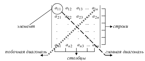
Числа 
Определение: Определителем II порядка называется число (выражение), записанное в виде квадратной таблицы размером 2×2, т.е. имеющая 2 строки и 2 столбца.
Определение: Определитель II порядка вычисляется по правилу: из произведения элементов, стоящих на главной диагонали, надо вычесть произведение элементов, стоящих на побочной диагонали: 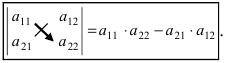
Пример:
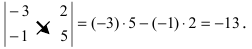
Определение: Определителем III порядка называется число (выражение), записанное в виде квадратной таблицы размером 3×3, то есть имеющей 3 строки и 3 столбца.
Определитель III порядка вычисляется по правилу Саррюса: за определителем выписывают первый и второй столбцы, затем из суммы произведений элементов, стоящих на главной диагонали ей параллельных диагоналях, надо вычесть сумму произведений элементов, стоящих на побочной диагонали и ей параллельных: 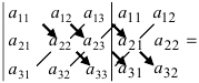

Пример:
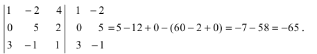
Определение: Минором  элемента
  называется определитель порядка (n-1), который получается из исходного определителя порядка n путем вычеркивания строки i и столбца j, на пересечении которых стоит элемент
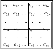
Пример:
Найти миноры элементов  и
и  определителя из Примера 2. Вычеркивая в определителе строку 1 и столбец 2:
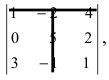 получим минор
 Поступая аналогично со строкой 3 и столбцом 3, получим минор
Пример:
Найти миноры элементов  и
и  определителя
  Исходя из определения минора
  получаем
  аналогично найдем минор
Определение: Алгебраическим дополнением  элемента
  называется произведение минора этого элемента на
  т.е.
т.е. 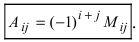
Замечание: Из определения алгебраического дополнения следует, что алгебраическое дополнение совпадает со своим минором, если сумма  является четным числом, и противоположно ему по знаку, если сумма — нечетное число.
Определение: Транспонированным определителем n-го порядка называется определитель порядка n, полученный из исходного определителя путем замены строк на соответствующие столбцы, а столбцов на соответствующие строки.
Если 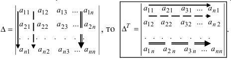
Пример:
Найти определитель, транспонированный к определителю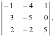 Из определения транспонированного определителя
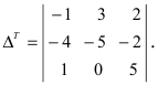
Свойства определителей
1. Величина транспонированного определителя равна величине исходного определителя. Пусть  Отсюда видно, что
2. Перестановка местами двух строк (столбцов) изменяет знак определителя на противоположный. Пусть 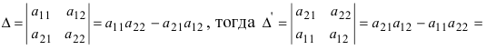
Если поменять местами строки (столбцы) четное число раз, то величина и знак определителя не меняется. Нечетная перестановка местами строк (столбцов) не меняет величину определителя, но изменяет его знак на противоположный.
3. Определитель, содержащий две (или более) одинаковых строки (столбца), равен нулю. Если определитель содержит два одинаковых столбца, то 
4. Для того чтобы умножить определитель на число k, достаточно умножить на это число все элементы какой-либо одной строки (столбца). Обратно: если все элементы какой-либо строки (столбца) имеют общий множитель k, то его можно вынести за знак определителя.
Докажем это свойство: 
5. Если две каких-либо строки (столбца) пропорциональны, то определитель равен нулю.
Пусть в определителе II порядка первая и вторая строки пропорциональны, тогда 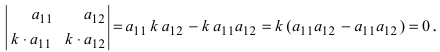
6. Если все элементы какой-либо строки (столбца) равны нулю, то определитель равен нулю.
Пусть в определителе II порядка все элементы первой строки равны нулю, тогда 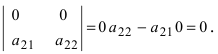
7. Если элементы какой-либо строки (или столбца) можно представить в виде двух слагаемых, то сам определитель можно представить в виде суммы двух определителей. Если 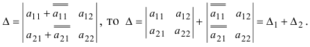 Доказать самостоятельно.
8. Если все элементы какой-либо строки (столбца) умножить на вещественное число к и прибавить k соответствующим элементам другой строки (соответственно, столбца), то величина определителя не изменится.
Умножим элементы второго столбца на вещественное число k и прибавим результат умножения к соответствующим элементам первого столбца, получим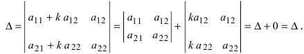
Второй определитель равен нулю по свойству 5.
Замечание: Данное свойство применяется для обнуления всех элементов какой-либо строки (столбца) за исключением одного (метод обнуления), что существенно снижает трудоемкость вычисления определителей порядка выше 3 (см. также свойство 9.).
9. [Метод раскрытия определителя по элементам какой-либо строки (или столбца); универсальный способ вычисления определителя любого порядка]. Определитель любого порядка равен сумме произведений элементов какой-либо строки (столбца) на их алгебраические дополнения:
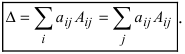
Пример:
Вычислить определитель 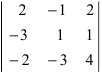 по элементам 3 строки и по элементам 2 столбца.
Решение:
Воспользуемся свойством 9.: раскроем определитель по элементам 3 строки 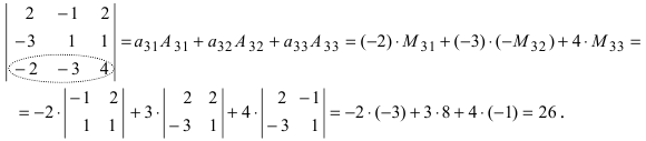 Вычислим определитель по элементам 2 столбца
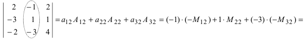
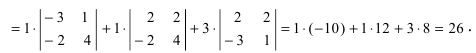
Из полученных результатов видно, что свойство 9. является универсальным методом вычисления любых определителей по элементам любой строки или столбца.
Используя свойство 8. можно обнулить все элементы какой-либо строки (столбца) за исключением одного (метод обнуления), а затем раскрыть определитель по элементам этой строки, воспользовавшись свойством 9.
Пример:
Вычислить определитель 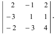
Решение:
Обнулим элементы в третьей строке, для чего выполним следующие действия: 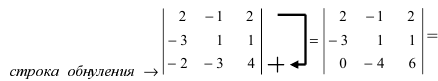 (по свойству 4. из третьей строки вынесем множитель 2)
 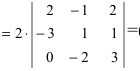 используя свойство 8., умножим все элементы второго столбца на 1.5 и прибавим к соответствующим элементам третьего столбца, получим)
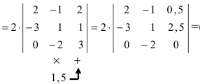
(по свойству 4. из третьего столбца вынесем множитель 0,5, тогда множитель перед определителем станет равным 1) 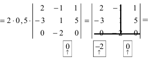
(раскроем определитель по элементам третьей строки: 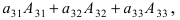 выше из определителя третьего порядка вычеркнута третья строка с нулями и второй столбец, т.е. показан необходимый для дальнейших вычислений минор
  Таким образом, метод обнуления позволяет значительно ускорить процесс вычисления любого определителя.
Пример:
Решить уравнение 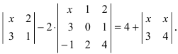
Решение:
Вычислим определители второго и третьего порядков согласно вышеописанным правилам:
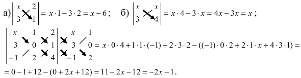
Найденные величины подставим в исходное уравнение

Пример:
Решить неравенство 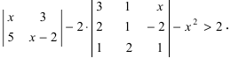
Решение:
Вычислим определители второго и третьего порядков согласно вышеописанным правилам: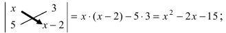
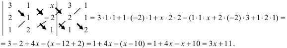
Найденные величины подставим в исходное неравенство 
Пример:
Вычислить определитель четвертого порядка (аналогично выполнить такие же действия с определителем третьего порядка), преобразовав его так, чтобы три элемента некоторого ряда равнялись нулю, и вычислить полученный определитель по элементам этого ряда: 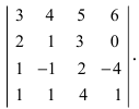
Решение:
Во второй строке исходного определителя присутствуют 1 и 0, поэтому обнуление элементов будем производить в этой строке (при обнулении элементов в строке действия производят со столбцами и наоборот): 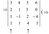 — строка обнуления;
  — столбцы, с которыми производят действия)=
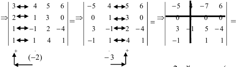
(по методу обнуления раскроем определитель по элементам 2-ой строки ( — цифры, с которыми производятся действия))

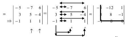 (по универсальному методу раскроем определитель по элементам третьей строки)

Определители
Перестановкой чисел 1, 2,…, n называется любое расположение этих чисел в определенном порядке. В элементарной алгебре доказывается, что число всех перестановок, которые можно образовать из n чисел, равно 12…n = n!. Например, из трех чисел 1, 2, 3 можно образовать 3!=6 перестановок: 123, 132, 312, 321, 231, 213. Говорят, что в данной перестановке числа i и j составляют инверсию (беспорядок), если i>j, но i стоит в этой перестановке раньше j, то есть если большее число стоит левее меньшего.
Перестановка называется четной (или нечетной), если в ней соответственно четно (нечетно) общее число инверсий. Операция, посредством которой от одной перестановки переходят к другой, составленной из тех же n чисел, называется подстановкой n-ой степени.
Подстановка, переводящая одну перестановку в другую, записывается двумя строками в общих скобках, причем числа, занимающие одинаковые места в рассматриваемых перестановках, называются соответствующими и пишутся одно под другим. Например, символ 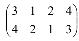 обозначает подстановку в которой 3 переходит в
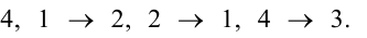
Подстановка называется четной (или нечетной), если общее число инверсий в обеих строках подстановки четно (нечетно). Всякая подстановка n-ой степени может быть записана в виде 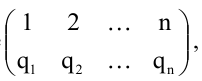 т.е. с натуральным расположением чисел в верхней строке.
Пусть нам дана квадратная матрица порядка n 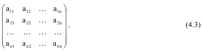
Рассмотрим все возможные произведения по n элементов этой матрицы, взятых по одному и только по одному из каждой строки и каждого столбца, т.е. произведений вида: 
где индексы  составляют некоторую перестановку из чисел 1, 2,…,n. Число таких произведений равно числу различных перестановок из n символов, т.е. равно n!. Знак произведения (4.4) равен (-1)q где q — число инверсий в перестановке вторых индексов элементов.
Определителем n-го порядка, соответствующим матрице (4.3), называется алгебраическая сумма n! членов вида (4.4). Для записи определителя употребляется символ 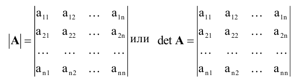 (детерминант, или определитель, матрицы А).
Свойства определителей:
- Определитель не меняется при транспонировании.
- Если одна из строк определителя состоит из нулей, то определитель равен нулю.
- Если в определителе переставить две строки, определитель поменяет знак.
- Определитель, содержащий две одинаковые строки, равен нулю.
- Если все элементы некоторой строки определителя умножить на некоторое число то сам определитель умножится на
- Определитель, содержащий две пропорциональные строки, равен нулю.
- Если все элементы i-й строки определителя представлены в виде суммы двух слагаемых то определитель равен сумме определителей, у которых все строки, кроме i-ой, — такие же, как в заданном определителе, а i-я строка в одном из слагаемых состоит из элементов в другом — из элементов
- Определитель не меняется, если к элементам одной из его строк прибавляются соответствующие элементы другой строки, умноженные на одно и то же число.
 то сам определитель умножится на
 то определитель равен сумме определителей, у которых все строки, кроме i-ой, — такие же, как в заданном определителе, а i-я строка в одном из слагаемых состоит из элементов
  в другом — из элементов
Замечание. Все свойства остаются справедливыми, если вместо строк взять столбцы.
Минором  элемента
  определителя d n-го порядка называется определитель порядка n-1, который получается из d вычеркиванием строки и столбца, содержащих данный элемент.
Алгебраическим дополнением элемента  определителя d называется его минор
  взятый со знаком
  Алгебраическое дополнение элемента
  будем обозначать
  Таким образом,
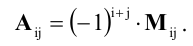
Способы практического вычисления определителей, основанные на том, что определитель порядка n может быть выражен через определители более низких порядков, дает следующая теорема.
- Заказать решение задач по высшей математике
Теорема (разложение определителя по строке или столбцу).
Определитель равен сумме произведений всех элементов произвольной его строки (или столбца) на их алгебраические дополнения. Иначе говоря, имеет место разложение d по элементам i-й строки  или j- го столбца
В частности, если все элементы строки (или столбца), кроме одного, равны нулю, то определитель равен этому элементу, умноженному на его алгебраическое дополнение.
Пример:
Не вычисляя определителя 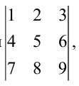 показать, что он равен нулю.
Решение:
Вычтем из второй строки первую, получим определитель 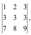 равный исходному. Если из третьей строки также вычесть первую, то получится определитель
 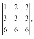 в котором две строки пропорциональны.
Такой определитель равен нулю.
Пример:
Вычислить определитель 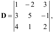 разложив его по элементам второго столбца.
Решение:
Разложим определитель по элементам второго столбца: 
Пример:
Вычислить определитель 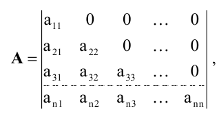 в котором все элементы по одну сторону от главной диагонали равны нулю.
Решение:
Разложим определитель А по первой строке:
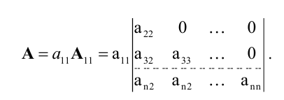
Определитель, стоящий справа, можно снова разложить по первой строке, тогда получим: 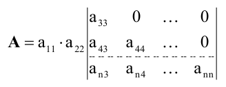
И так далее. После n шагов придем к равенству 
Пример:
Вычислить определитель 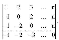
Решение:
Если к каждой строке определителя, начиная со второй, прибавить первую строку, то получится определитель, в котором все элементы, находящиеся ниже главной диагонали, будут равны нулю. А именно, получим определитель: 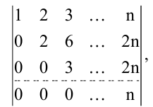 равный исходному.
Рассуждая, как в предыдущем примере найдем, что он равен произведению элементов главной диагонали, т.е. n!. Способ, с помощью которого вычислен данный определитель, называется способом приведения к треугольному виду.
——- в вышмате
Определители. Алгебраические дополнения
Внимание! Понятие определителя вводится только для квадратной матрицы.
Матрица называется квадратной порядка n, если количество ее строк совпадает с количеством столбцов и равно n.
Элементы квадратной матрицы, имеющие одинаковые значения индексов, составляют главную диагональ. Элементы квадратной матрицы порядка n, сумма индексов каждого из которых равна n+1, составляют побочную диагональ.
Определитель матрицы  обозначается одним из следующих символов:
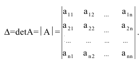
Внимание! Определитель — это число, характеризующее квадратную мат- рицу.
Определитель матрицы второго порядка равен разности элементов главной и побочной диагоналей соответственно:
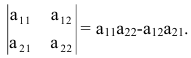
Определитель матрицы третьего порядка равен сумме элементов главной диагонали и элементов, расположенных в вершинах треугольников с основаниями, параллельными главной диагонали, а также разности элементов побочной диагонали и элементов, расположенных в вершинах треугольников с основаниями, параллельными побочной диагонали. 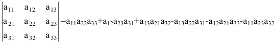
Схематично это правило изображается так (правило треугольника): 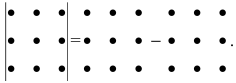
Например,
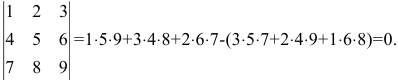 Квадратная матрица называется верхней (нижней) треугольной, если все элементы, стоящие под (над) главной диагональю равны нулю.
Отметим некоторые свойства определителя.
- Определитель треугольной матрицы равен произведению элементов главной диагонали.
- При транспонировании матрицы ее определитель не изменяется.
- От перестановки двух рядов (строк или столбцов) определитель меняет знак.
- Общий множитель всех элементов некоторого ряда определителя можно выносить за знак определителя.
- Если все элементы какого-нибудь ряда матрицы равны нулю, то определитель равен нулю.
- Определитель, содержащий два пропорциональных ряда, равен нулю.
- Определитель не изменится, если к элементам какого-либо ряда прибавить соответствующие элементы другого ряда, умноженные на одно и то же число.
- Определитель произведения двух матриц одинакового порядка равен произведению определителей этих матриц.
Минором элемента  определителя n-го порядка называется определитель (n-l)-ro порядка, получаемый вычеркиванием i-й строки и j-ro столбца, на пересечении которых стоит этот элемент. Обозначение:
Алгебраическим дополнением элемента  называется его минор, умноженный на
  Обозначение:
Теорема разложения.
Определитель матрицы равен сумме произведений элементов любого ряда на их алгебраические дополнения.
Пример №2
Вычислить определитель, разлагая его по элементам первой строки: 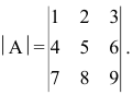
Решение:
По теореме разложения 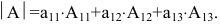
Найдем алгебраические дополнения элементов матрицы А: 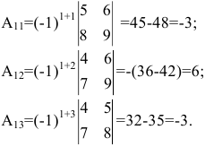
Следовательно,
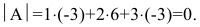
Для вычисления определителя порядка выше третьего удобно пользоваться теоремой разложения (метод понижения порядка) или методом приведения определителя к треугольному виду.
Пример №3
Вычислить определитель, приведя его к треугольному виду:
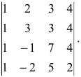
Решение:
Применяя свойство 6 определителей, преобразуем последовательно второй, третий, четвертый столбцы матрицы. 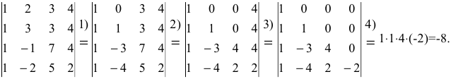
- прибавили ко второму столбцу первый, умноженный на -2;
- прибавили к третьему столбцу первый, умноженный на -3;
- прибавили к четвертому столбцу первый, умноженный на -4;
- применили свойство 1 определителей.
- Критерий совместности Кронекера-Капелли
- Формулы Крамера
- Матричный метод
- Экстремум функции
- Пределы в математике
- Функции многих переменных
- Уравнения прямых и кривых на плоскости
- Плоскость и прямая в пространстве
Определитель матрицы.
Навигация по странице:
- Определение определителя матрицы
- Свойства определителя матрицы
- Методы вычисления определителя матрицы
- Определитель матрицы 1×1
- Определитель матрицы 2×2
- Определитель матрицы 3×3
- Правило треугольника для вычисления определителя матрицы 3-тего порядка
- Правило Саррюса для вычисления определителя матрицы 3-тего порядка
- Определитель матрицы произвольного размера
- Разложение определителя по строке или столбцу
- Приведение определителя к треугольному виду
- Теорема Лапласа
Определитель матрицы или детерминант матрицы — это одна из основных численных характеристик квадратной матрицы, применяемая при решении многих задач.
Определение.
Определителем матрицы n×n будет число:
| det(A) = | Σ | (-1)N(α1,α2,…,αn)·aα11·aα22·…·aαnn |
| (α1,α2,…,αn) |
где (α1,α2,…,αn) — перестановка чисел от 1 до n, N(α1,α2,…,αn) — число инверсий в перестановке, суммирование идёт по всем возможным перестановкам порядка n.
Обозначение
Определитель матрици A обычно обозначается det(A), |A|, или ∆(A).
Свойства определителя матрицы
-
Определитель матрицы с двумя равными строками (столбцами) равен нулю.
-
Определитель матрицы с двумя пропорциональными строками (столбцами) равен нулю.
-
Определитель матрицы, содержащий нулевую строку (столбец), равен нулю.
-
Определитель матрицы равен нулю если две (или несколько) строк (столбцев) матрицы линейно зависимы.
-
При транспонировании значение определителя матрицы не меняется:
det(A) = det(AT)
-
Определитель обратной матрицы:
det(A-1) = det(A)-1
-
Определитель матрицы не изменится, если к какой-то его строке (столбцу) прибавить другую строку (столбец), умноженную на некоторое число.
-
Определитель матрицы не изменится, если к какой-то его строке (столбцу) прибавить линейную комбинации других строк (столбцов).
-
Если поменять местами две строки (столбца) матрицы, то определитель матрицы поменяет знак.
-
Общий множитель в строке (столбце) можно выносить за знак определителя:
a11a12…a1n
a21a22…a2n
….
k·ai1k·ai2…k·ain
….
an1an2…ann=
k·
a11a12…a1n
a21a22…a2n
….
ai1ai2…ain
….
an1an2…ann
-
Если квадратная матрица n-того порядка умножается на некоторое ненулевое число, то определитель полученной матрицы равен произведению определителя исходной матрицы на это число в n-той степени:
B = k·A => det(B) = kn·det(A)
где A матрица n×n, k — число.
-
Если каждый элемент в какой-то строке определителя равен сумме двух слагаемых, то исходный определитель равен сумме двух определителей, в которых вместо этой строки стоят первые и вторые слагаемые соответственно, а остальные строки совпадают с исходным определителем:
a11a12…a1n
a21a22…a2n
….
bi1 + ci1bi2 + ci2…bin + cin
….
an1an2…ann=
a11a12…a1n
a21a22…a2n
….
bi1bi2…bin
….
an1an2…ann+
a11a12…a1n
a21a22…a2n
….
ci1ci2…cin
….
an1an2…ann -
Определитель верхней (нижней) треугольной матрицы равен произведению его диагональных элементов.
-
Определитель произведения матриц равен произведению определителей этих матриц:
det(A·B) = det(A)·det(B)
Методы вычисления определителя матрицы
Вычисление определителя матрицы 1×1
Правило:
Для матрицы первого порядка значение определителя равно значению элемента этой матрицы:
∆ = |a11| = a11
Вычисление определителя матрицы 2×2
Правило:
Для матрицы 2×2 значение определителя равно разности произведений элементов главной и побочной диагоналей:
| ∆ = |
|
= a11·a22 — a12·a21 |
Пример 1.
Найти определитель матрицы A
Решение:
| det(A) = |
|
= 5·1 — 7·(-4) = 5 + 28 = 33 |
Вычисление определителя матрицы 3×3
Правило треугольника для вычисления определителя матрицы 3-тего порядка
Правило:
Для матрицы 3×3 значение определителя равно сумме произведений элементов главной диагонали и произведений элементов лежащих на треугольниках с гранью параллельной главной диагонали, от которой вычитается произведение элементов побочной диагонали и произведение элементов лежащих на треугольниках с гранью параллельной побочной диагонали.
| ∆ = |
|
= |
=
a11·a22·a33 +
a12·a23·a31 +
a13·a21·a32 —
a13·a22·a31 —
a11·a23·a32 —
a12·a21·a33
Правило Саррюса для вычисления определителя матрицы 3-тего порядка
Правило:
Справа от определителя дописывают первых два столбца и произведения элементов на главной диагонали и на диагоналях, ей параллельных, берут со знаком «плюс»; а произведения элементов побочной диагонали и диагоналей, ей параллельных, со знаком «минус»:
| ∆ = |
|
= |
=
a11·a22·a33 +
a12·a23·a31 +
a13·a21·a32 —
a13·a22·a31 —
a11·a23·a32 —
a12·a21·a33
Пример 2.
Найти определитель матрицы A =
571
-410
203
Решение:
det(A) =
571
-410
203
=
5·1·3 + 7·0·2 + 1·(-4)·0 —
1·1·2 — 5·0·0 — 7·(-4)·3 = 15 + 0 + 0 — 2 — 0 + 84 = 97
Вычисление определителя матрицы произвольного размера
Разложение определителя по строке или столбцу
Правило:
Определитель матрицы равен сумме произведений элементов строки определителя на их алгебраические дополнения:
| n | |||
| det(A) = | Σ | aij·Aij | — разложение по i-той строке |
| j = 1 |
Правило:
Определитель матрицы равен сумме произведений элементов столбца определителя на их алгебраические дополнения:
| n | |||
| det(A) = | Σ | aij·Aij | — разложение по j-тому столбцу |
| i = 1 |
При разложение определителя матрицы обычно выбирают ту строку/столбец, в которой/ом максимальное количество нулевых элементов.
Пример 3.
Найти определитель матрицы A
Решение: Вычислим определитель матрицы разложив его по первому столбцу:
| det(A) = |
|
= |
= 2·(-1)1+1·
21
11
+ 0·(-1)2+1·
41
11
+ 2·(-1)3+1·
41
21
=
= 2·(2·1 — 1·1) + 2·(4·1 — 2·1) = 2·(2 — 1) + 2·(4 — 2) = 2·1 + 2·2 = 2 + 4 = 6
Пример 4.
Найти определитель матрицы A
Решение: Вычислим определитель матрицы, разложив его по второй строке (в ней больше всего нулей):
det(A) =
2411
0200
2113
4023
=
— 0·
411
113
023
+ 2·
211
213
423
— 0·
241
213
403
+ 0·
241
211
402
=
= 2·(2·1·3 + 1·3·4 + 1·2·2 — 1·1·4 — 2·3·2 — 1·2·3) = 2·(6 +12 + 4 — 4 — 12 — 6) = 2·0 = 0
Приведение определителя к треугольному виду
Правило:
Используя свойства определителя для элементарных преобразований над строками и столбцами 8 — 11, определитель приводится к треугольному виду, и тогда его значение будет равно произведению элементов стоящих на главной диагонали.
Пример 5.
Найти определитель матрицы A приведением его к треугольному виду
Решение:
det(A) =
2411
0210
2113
4023
Сначала получим нули в первом столбце под главной диагональю. Для этого отнимем от 3-тей строки 1-ую строку, а от 4-той строки 1-ую строку, умноженную на 2:
det(A) =
2411
0210
2 — 21 — 41 — 13 — 1
4 — 2·20 — 4·22 — 1·23 — 1·2
=
2411
0210
0-302
0-801
Получим нули во втором столбце под главной диагональю. Для этого поменяем местами 2-ой и 3-тий столбцы (при этом детерминант сменит знак на противоположный):
det(A) = —
2141
0120
00-32
00-81
Получим нули в третьем столбце под главной диагональю. Для этого к 3-ему столбцу добавим 4-тий столбец, умноженный на 8:
det(A) = —
214 + 1·81
012 + 0·80
00-3 + 2·82
00-8 + 1·81
=
—
21121
0120
00132
0001
= -2·1·13·1 = -26
Теорема Лапласа
Теорема:
Пусть ∆ — определитель n-ого порядка. Выберем в нем произвольные k строк (столбцов), причем k < n. Тогда сумма произведений всех миноров k-ого порядка, которые содержатся в выбранных строках (столбцах), на их алгебраические дополнения равна определителю.
Определитель матрицы
Определителем
квадратной матрицы
![]() называется число, которое обозначается
называется число, которое обозначается
как![]() или
или![]() и вычисляется при помощи следующих трех
и вычисляется при помощи следующих трех
правил.
Правило
1.
Определитель диагональной матрицы
равен произведению элементов, стоящих
на главной диагонали.
Замечание:
Определитель одноэлементной матрицы
равен самому элементу.
Правило
2.
Общий множитель элементов любой строки
или столбца матрицы можно вынести за
знак определителя.
Замечание:
Определитель матрицы, у которой строка
или столбец состоит только из нулей,
равен
![]() .
.
Правило
3.
Определитель матрицы не изменится, если
к одной из строк (столбцов) матрицы
прибавить другую строку (столбец) этой
матрицы.
Свойства определителя матрицы.
1.
Определитель не меняется при
транспонировании.
2. Если
в определителе переставить две строки,
определитель поменяет знак.
3.
Определитель, содержащий две одинаковые
строки, равен нулю.
4.
Определитель, содержащий две
пропорциональные строки, равен нулю.
5. Если
все элементы
![]() строки определителя представлены в
строки определителя представлены в
виде суммы двух слагаемых![]() ,
,
то определитель равен сумме определителей,
у которых все строки, кроме![]() ,
,
— такие же, как в заданном определителе,
а![]() строка в одном из слагаемых состоит из
строка в одном из слагаемых состоит из
элементов![]() ,
,
в другом — из элементов![]() .
.
Замечание.
Все свойства остаются справедливыми,
если вместо строк взять столбцы.
Миноры и алгебраические дополнения
Обозначим
через
![]() матрицу, которая остается при вычеркивании
матрицу, которая остается при вычеркивании
из матрицы![]()
![]() строки и
строки и![]() столбца. Тогда
столбца. Тогда![]() называется минором элемента
называется минором элемента![]() .
.
Величина![]() называется алгебраическим дополнением
называется алгебраическим дополнением
элемента![]() .
.
Разложение определителя матрицы по элементам строки или столбца.
Теорема.
Определитель каждой матрицы равен сумме
произведений элементов любой ее строки
(столбца) на их алгебраические дополнения,
т. е. при разложении по элементам
![]() строки
строки

Для
вычисления значений определителей
матриц второго порядка пользуются
формулой:
![]()
Для
вычисления значений определителей
матриц третьего порядка можно
воспользоваться формулой разложения
определителя по первой строке:

Пример
7.
Не
вычисляя определителя
 ,
,
показать, что он равен нулю.
Решение.
Вычтем
из второй строки первую, получим
определитель
 ,
,
равный исходному. Если из третьей
строки также вычесть первую, то получится
определитель
 ,
,
в котором две строки пропорциональны.
Такой определитель равен нулю.
Пример
8.
Вычислить
определитель
 ,
,
разложив его по элементам второго
столбца.
Решение.
Разложим
определитель по элементам второго
столбца:

4. Ранг матрицы
Рассмотрим
прямоугольную матрицу
![]() .
.
Если в этой матрице выделить произвольно![]() строк и
строк и![]() столбцов, то элементы, стоящие на
столбцов, то элементы, стоящие на
пересечении выделенных строк и столбцов,
образуют квадратную матрицу![]() порядка. Определитель этой матрицы
порядка. Определитель этой матрицы
называетсяминором
k-го порядка матрицы
![]() .
.
Очевидно, что матрица![]() обладает минорами любого порядка от
обладает минорами любого порядка от![]() до наименьшего из чисел
до наименьшего из чисел![]() и
и![]() .
.
Некоторые среди них будут равны нулю.
Среди всех отличных от нуля миноров
матрицы![]() найдется, по крайней мере, один минор,
найдется, по крайней мере, один минор,
порядок которого будет наибольшим.
Наибольший из порядков миноров данной
матрицы, отличных от нуля, называется
рангом
матрицы. Если ранг
матрицы
![]() равен
равен![]() ,
,
то это означает, что в матрице![]() имеется отличный от нуля минор порядка
имеется отличный от нуля минор порядка![]() ,
,
но всякий минор порядка, большего чем![]() ,
,
равен нулю. Ранг матрицы![]() обозначается через
обозначается через![]() .
.
Очевидно, что выполняется соотношение
![]()
Ранг
матрицы находится либо методом окаймления
миноров, либо методом элементарных
преобразований. При вычислении ранга
матрицы первым способом следует
переходить от миноров низших порядков
к минорам более высокого порядка. Если
уже найден минор
![]()
![]() порядка матрицы
порядка матрицы![]() ,
,
отличный от нуля, то требуют вычисления
лишь миноры![]() порядка, окаймляющие минор
порядка, окаймляющие минор![]() ,
,
т.е. содержащие его в качестве минора.
Если все они равны нулю, то ранг матрицы
равен![]() .
.
Элементарными
называются следующие преобразования
матрицы:
-
перестановка
двух любых строк (или столбцов), -
умножение
строки (или столбца) на отличное от нуля
число, -
прибавление
к одной строке (или столбцу) другой
строки (или столбца), умноженной на
некоторое число.
Две
матрицы называются
эквивалентными,
если одна из них получается из другой
с помощью конечного множества элементарных
преобразований.
Эквивалентные
матрицы не являются, вообще говоря,
равными, но их ранги равны. Если матрицы
![]() и
и
![]()
эквивалентны, то это записывается так:
![]() .
.
Каноническойматрицей называется матрица, у которой
в начале главной диагонали стоят подряд
несколько единиц (число которых может
равняться нулю), а все остальные элементы
равны нулю, например,
 .
.
При
помощи элементарных преобразований
строк и столбцов любую матрицу можно
привести к канонической. Ранг канонической
матрицы равен числу единиц на ее главной
диагонали.
Пример
11.
Найти методом окаймления миноров ранг
матрицы

Решение.
Начинаем
с миноров
![]() порядка, (т.е. с элементов матрицы
порядка, (т.е. с элементов матрицы![]() ).
).
Выберем, например, минор (элемент)![]() ,
,
расположенный в первой строке и первом
столбце. Окаймляя при помощи второй
строки и третьего столбца, получаем
минор![]() ,
,
отличный от нуля. Переходим теперь к
минорам![]() порядка, окаймляющим
порядка, окаймляющим![]() .
.
Их всего два (можно добавить второй
столбец или четвертый). Вычисляем их:
 ,
,
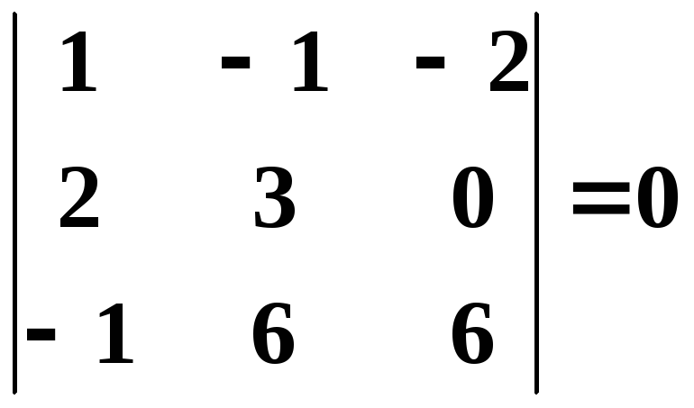 .
.
Таким
образом, все окаймляющие миноры третьего
порядка оказались равными нулю. Ранг
матрицы
![]() равен двум.
равен двум.
Пример
12.
Найти ранг матрицы

и
привести ее к каноническому виду.
Решение. Из второй строки
вычтем первую и переставим эти строки:
 .
.
Теперь из второй и третьей
строк вычтем первую, умноженную
соответственно на
![]() и
и![]() :
:
 ;
;
из третьей строки вычтем
вторую, при этом получим матрицу
 ,
,
которая эквивалентна матрице
![]() ,
,
так как получена из нее с помощью
конечного множества элементарных
преобразований. Очевидно, что ранг
матрицы![]() равен
равен![]() ,
,
а следовательно, и![]() .
.
Матрицу
![]() легко привести к канонической.
легко привести к канонической.
Вычитая первый столбец,
умноженный на подходящие числа, из всех
последующих, обратим в нуль все элементы
первой строки, кроме первого, причем
элементы остальных строк не изменяются.

Затем, вычитая второй
столбец, умноженный на подходящие числа,
из всех последующих, обратим в нуль все
элементы второй строки, кроме второго,
и получим каноническую матрицу:
.
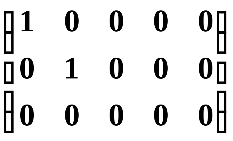
Соседние файлы в папке Лекц.Мат-ка Базов
- #
- #
- #
- #
- #
- #

Эксперт по предмету «Математика»
Задать вопрос автору статьи
Любой квадратной матрице $A=left(a_{ij} right)_{ntimes n} $ можно сопоставить некоторое число, которое будем называть определителем данной матрицы (детерминант).
Для обозначения определителя матрицы используют следующие символы: $|A|,, Delta $ или $det A$.
В зависимости от порядка матрицы различают несколько способов вычисления определителя.
Определитель матрицы 2-го порядка можно вычислить по формуле:
Пример 1
Дана матрица $A=left(begin{array}{cc} {1} & {-2} \ {3} & {1} end{array}right)$. Найти определитель.
Решение:
[det A=left|begin{array}{cc} {1} & {-2} \ {3} & {1} end{array}right|=1cdot 1-3cdot (-2)=1+6=7]
Для нахождения определителя матрицы 3-го порядка можно использовать одно из двух правил:
- правило треугольника;
- правило Саррюса.
Определитель матрицы 3-го порядка с помощью правила треугольника вычисляется по формуле:
[left|begin{array}{ccc} {a_{11} } & {a_{12} } & {a_{13} } \ {a_{21} } & {a_{22} } & {a_{23} } \ {a_{31} } & {a_{32} } & {a_{33} } end{array}right|=]
[=a_{11} cdot a_{22} cdot a_{33} +a_{31} cdot a_{12} cdot a_{23} +a_{21} cdot a_{32} cdot a_{13} -a_{31} cdot a_{22} cdot a_{13} -a_{21} cdot a_{12} cdot a_{33} -a_{11} cdot a_{23} cdot a_{32} ]
Для лучшего запоминания правила треугольника можно пользоваться следующей схемой:
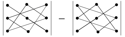
Пример 2
Дана матрица $A=left(begin{array}{ccc} {1} & {3} & {4} \ {0} & {2} & {1} \ {1} & {5} & {-1} end{array}right)$. Найти определитель.
Решение:
[begin{array}{l} {det A=left|begin{array}{ccc} {1} & {3} & {4} \ {0} & {2} & {1} \ {1} & {5} & {-1} end{array}right|=1cdot 2cdot (-1)+1cdot 3cdot 1+4cdot 0cdot 5-1cdot 2cdot 4-0cdot 3cdot (-1)-5cdot 1cdot 1=} \ {=-2+3+0-8-0-5=-12} end{array}]
Для вычисления определителя по правилу Саррюса необходимо выполнить следующие действия:
- дописать слева от определителя для первых столбца;
- перемножить элементы, расположенные на главной диагонали и параллельных ей диагоналях, взяв произведения со знаком «+»;
- перемножить элементы побочной диагонали и параллельных ей диагоналей, взяв произведения со знаком «-»
[left|begin{array}{ccc} {a_{11} } & {a_{12} } & {a_{13} } \ {a_{21} } & {a_{22} } & {a_{23} } \ {a_{31} } & {a_{32} } & {a_{33} } end{array}right|=]
[=a_{11} cdot a_{22} cdot a_{33} +a_{12} cdot a_{23} cdot a_{31} +a_{13} cdot a_{21} cdot a_{32} -a_{13} cdot a_{22} cdot a_{31} -a_{11} cdot a_{23} cdot a_{32} -a_{12} cdot a_{21} cdot a_{33} ]
Для лучшего запоминания правила треугольника можно пользоваться следующей схемой:
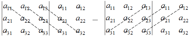
«Определитель матрицы и его вычисление» 👇
Пример 3
Дана матрица $A=left(begin{array}{ccc} {1} & {3} & {4} \ {0} & {2} & {1} \ {-2} & {5} & {-1} end{array}right)$. Найти определитель.
Решение:
[begin{array}{l} {A=left|begin{array}{ccc} {1} & {3} & {4} \ {0} & {2} & {1} \ {-2} & {5} & {-1} end{array}right|, , , begin{array}{c} {1} \ {0} \ {-2} end{array}, , , , begin{array}{c} {3} \ {2} \ {5} end{array}=1cdot 2cdot (-1)+3cdot 1cdot (-2)+4cdot 0cdot 5-4cdot 2cdot (-2)-1cdot 1cdot 5-3cdot 0cdot (-1)=} \ {=-2-6+0+16-5-0=3} end{array}]
Для вычисления определителя матрицы 4-го порядка и выше можно использовать один из двух способов:
- разложение по элементам строки;
- разложение по элементам столбца.
Данные способы сводят вычисление определителя порядка $n$ к вычислению определителя порядка $n-1$ за счет представления определителя суммой произведений элементов строки (столбца) на их алгебраические дополнения.
Разложение определителя матрицы по элементам строки в общем виде можно записать по формуле:
[det A=a_{i1} cdot A_{i1} +a_{i2} cdot A_{i2} +…+a_{in} cdot A_{in} ]
Разложение определителя матрицы по элементам столбца в общем виде можно записать по формуле:
[det A=a_{1j} cdot A_{1j} +a_{2j} cdot A_{2j} +…+a_{nj} cdot A_{nj} ]
Замечание 1
При разложении определителя по элементам строки (столбца) желательно выбирать строку (столбец), в которой(-ом) есть нули.
Пример 3
Дана матрица $A=left(begin{array}{cccc} {0} & {1} & {-1} & {3} \ {2} & {1} & {0} & {0} \ {-2} & {4} & {5} & {1} \ {3} & {2} & {1} & {0} end{array}right)$. Записать разложение определителя по произвольной строке (столбцу).
Решение:
- разложение по второй строке:
- разложение по четвертому столбцу:
[A=left|begin{array}{cccc} {0} & {1} & {-1} & {3} \ {2} & {1} & {0} & {0} \ {-2} & {4} & {5} & {1} \ {3} & {2} & {1} & {0} end{array}right|=2cdot (-1)^{3} cdot left|begin{array}{ccc} {1} & {-1} & {3} \ {4} & {5} & {1} \ {2} & {1} & {0} end{array}right|+1cdot (-1)^{4} cdot left|begin{array}{ccc} {0} & {-1} & {3} \ {-2} & {5} & {1} \ {3} & {1} & {0} end{array}right|=-2cdot left|begin{array}{ccc} {1} & {-1} & {3} \ {4} & {5} & {1} \ {2} & {1} & {0} end{array}right|+1cdot left|begin{array}{ccc} {0} & {-1} & {3} \ {-2} & {5} & {1} \ {3} & {1} & {0} end{array}right|]
[A=left|begin{array}{cccc} {0} & {1} & {-1} & {3} \ {2} & {1} & {0} & {0} \ {-2} & {4} & {5} & {1} \ {3} & {2} & {1} & {0} end{array}right|=3cdot (-1)^{5} cdot left|begin{array}{ccc} {2} & {1} & {0} \ {-2} & {4} & {5} \ {3} & {2} & {1} end{array}right|+1cdot (-1)^{7} cdot left|begin{array}{ccc} {0} & {1} & {-1} \ {2} & {1} & {0} \ {3} & {2} & {1} end{array}right|=-3cdot left|begin{array}{ccc} {2} & {1} & {0} \ {-2} & {4} & {5} \ {3} & {2} & {1} end{array}right|-1cdot left|begin{array}{ccc} {0} & {1} & {-1} \ {2} & {1} & {0} \ {3} & {2} & {1} end{array}right|]
Свойства определителя:
- элементарные преобразования строк (столбцов) матрицы не меняют значения определителя;
- перестановка строк (столбцов) меняет знак определителя на противоположный (c «+» на «-» и наоборот);
- определитель треугольной матрицы находится как произведение элементов, которые расположены на главной диагонали.
Пример 4
Дана матрица $A=left(begin{array}{ccc} {1} & {3} & {4} \ {0} & {2} & {1} \ {0} & {0} & {5} end{array}right)$. Найти определитель.
Решение:
[det A=left|begin{array}{ccc} {1} & {3} & {4} \ {0} & {2} & {1} \ {0} & {0} & {5} end{array}right|=1cdot 2cdot 5=10]
Замечание 2
Определитель матрицы, содержащей нулевую строку, равен нулю.
Замечание 3
Определитель матрицы, содержащей нулевой столбец, равен нулю.
Находи статьи и создавай свой список литературы по ГОСТу
Поиск по теме
Мы уже знакомы с понятием определителя матрицы. Было рассмотрено вычисление определителей первого, второго, третьего и высших порядков. Познакомимся со свойствами определителей, позволяющими значительно упростить их вычисление.
Под рядами определителя будем понимать строки и столбцы.
Свойства определителя матрицы
Значение определителя останется прежним, если заменить его строки столбцами (т.е. при транспонировании).
Это свойство можно обозначить следующим образом: ∣A∣=∣AT∣|A|=|A^{T}|. В общем виде оно выглядит так:
∣a11a12…a1na21a22…a2n…………am1am2…amn∣=∣a11a21…am1a12a22…am2…………a1na2n…amn∣begin{vmatrix}a_{11}&a_{12}&…&a_{1n}\a_{21}&a_{22}&…&a_{2n}\…&…&…&…\a_{m1}&a_{m2}&…&a_{mn}end{vmatrix}=begin{vmatrix}a_{11}&a_{21}&…&a_{m1}\a_{12}&a_{22}&…&a_{m2}\…&…&…&…\a_{1n}&a_{2n}&…&a_{mn}end{vmatrix}.
Пример 1
∣1015142∣=∣1014152∣=−190begin{vmatrix}10&15\14&2end{vmatrix}=begin{vmatrix}10&14\15&2end{vmatrix}=-190.
Пример 2
∣1011−73−814151921∣=∣1031511−819−71421∣=−3962begin{vmatrix}10&11&-7\3&-8&14\15&19&21end{vmatrix}=begin{vmatrix}10&3&15\11&-8&19\-7&14&21end{vmatrix}=-3962.
Если переставить два параллельных ряда, то определитель изменит свой знак.
Пример 1
Переставим местами строки №1 и №3 и вычислим определитель:
∣−1529−371914−11−5−128∣=−∣−5−1281914−11−1529−37∣=3333begin{vmatrix}-15&29&-37\19&14&-11\-5&-12&8end{vmatrix}=-begin{vmatrix}-5&-12&8\19&14&-11\-15&29&-37end{vmatrix}=3333.
Пример 2
Переставим местами столбцы №1 и №2 и вычислим определитель:
∣−1529−371914−11−5−128∣=−∣29−15−371419−11−12−58∣=3333begin{vmatrix}-15&29&-37\19&14&-11\-5&-12&8end{vmatrix}=-begin{vmatrix}29&-15&-37\14&19&-11\-12&-5&8end{vmatrix}=3333.
Определитель равен нулю, если среди его рядов есть два одинаковых ряда.
Пример 1
Определитель содержит две одинаковые строки: №1 и №3:
∣111792514211179∣=0begin{vmatrix}11&17&9\25&14&2\11&17&9end{vmatrix}=0.
Пример 2
Определитель содержит два одинаковых столбца: №1 и №2:
∣252545191934393922∣=0begin{vmatrix}25&25&45\19&19&34\39&39&22end{vmatrix}=0.
Определитель равен нулю, если среди его рядов есть два пропорциональных ряда.
Пример 1
Определитель содержит две пропорциональных строки – №1 и №3:
∣1015265711203052∣=0begin{vmatrix}10&15&26\5&7&11\20&30&52end{vmatrix}=0.
Пример 2
Определитель содержит два пропорциональных столбца – №2 и №3:
∣539154129721∣=0begin{vmatrix}5&3&9\15&4&12\9&7&21end{vmatrix}=0.
Определитель, содержащий ряд, состоящий из нулей, равен нулю.
Пример 1
∣11825000191432∣=0begin{vmatrix}11&8&25\0&0&0\19&14&32end{vmatrix}=0.
Пример 2
∣91702514013160∣=0begin{vmatrix}9&17&0\25&14&0\13&16&0end{vmatrix}=0.
Общий множитель элементов какого-либо ряда определителя можно вынести за знак определителя.
Пример 1
Вынесем общий множитель — 5 из строки №2 и вычислим определитель:
∣19153752540131810∣=5⋅∣191537158131810∣=5⋅(−2115)=−10575begin{vmatrix}19&15&37\5&25&40\13&18&10end{vmatrix}=5cdotbegin{vmatrix}19&15&37\1&5&8\13&18&10end{vmatrix}=5cdot(-2115)=-10575.
Пример 2
Вынесем общий множитель — число 7 из столбца №1 и вычислим определитель:
∣7281114139211045∣=7⋅∣12811213931045∣=7⋅(−1478)=−10346begin{vmatrix}7&28&11\14&13&9\21&10&45end{vmatrix}=7cdotbegin{vmatrix}1&28&11\2&13&9\3&10&45end{vmatrix}=7cdot(-1478)=-10346.
В случае если все элементы некоторого ряда определителя представимы в виде суммы двух слагаемых, то определитель может быть записан как сумма двух определителей, у которых элементы рассматриваемого ряда равны соответствующим слагаемым, а остальные элементы одни и те же.
Пример 1
Представим в виде суммы двух слагаемых элементы второй строки и вычислим определитель:
∣135268351∣=∣1351+14+25+3351∣=∣135145351∣+∣135123351∣=−14+6=−8begin{vmatrix}1&3&5\2&6&8\3&5&1end{vmatrix}=begin{vmatrix}1&3&5\1+1&4+2&5+3\3&5&1end{vmatrix}=begin{vmatrix}1&3&5\1&4&5\3&5&1end{vmatrix}+begin{vmatrix}1&3&5\1&2&3\3&5&1end{vmatrix}=-14+6=-8.
Пример 2
Представим в виде суммы двух слагаемых элементы столбца №2 и вычислим определитель:
∣153168351∣=∣12+3313+3832+31∣=∣123138321∣+∣133138331∣=12+30=42begin{vmatrix}1&5&3\1&6&8\3&5&1end{vmatrix}=begin{vmatrix}1&2+3&3\1&3+3&8\3&2+3&1end{vmatrix}=begin{vmatrix}1&2&3\1&3&8\3&2&1end{vmatrix}+begin{vmatrix}1&3&3\1&3&8\3&3&1end{vmatrix}=12+30=42.
Значение определителя останется прежним, если к элементам одного ряда прибавить соответствующие элементы другого ряда, предварительно умножив их на любое число.
Пример 1
К элементам строки №3 прибавим элементы строки №1, умноженные на -3:
∣13−22−1132−5∣=∣13−22−110−71∣=28begin{vmatrix}1&3&-2\2&-1&1\3&2&-5end{vmatrix}=begin{vmatrix}1&3&-2\2&-1&1\0&-7&1end{vmatrix}=28.
Пример 2
К элементам столбца №3 прибавим элементы столбца №1, умноженные на -4:
∣154248351∣=∣15024035−11∣=66begin{vmatrix}1&5&4\2&4&8\3&5&1end{vmatrix}=begin{vmatrix}1&5&0\2&4&0\3&5&-11end{vmatrix}=66.
Данные свойства могут применяться для нахождения определителей любого порядка. Их знание и применение значительно упростит процесс вычисления детерминантов.
Наши эксперты помогут вам решить контрольную работу онлайн по любому предмету!