Определение силы сопротивления в физике и её формула
Содержание:
-
Что такое сила сопротивления в физике
- От чего зависит в механике и динамике
-
Разновидности сил сопротивления
- Сила сопротивления качению
- Сила сопротивления воздуха
- Как найти трение
- Силы сопротивления при больших скоростях
Что такое сила сопротивления в физике
Сила сопротивления — сила, которая возникает во время движения тела в жидкой или газообразной среде и препятствует этому движению.
Важно уметь отличать силу сопротивления от силы трения. Во втором случае рассматривается характер взаимодействия твердых тел друг с другом. Таким образом, трение можно наблюдать, когда какой-либо предмет перемещается по поверхности другого. Вектор этой силы будет направлен в противоположную сторону направления движения.
Для того чтобы рассчитать силу сопротивления необходимо умножить коэффициент сопротивления материала на силу, провоцирующую перемещение этого предмета.
Осторожно! Если преподаватель обнаружит плагиат в работе, не избежать крупных проблем (вплоть до отчисления). Если нет возможности написать самому, закажите тут.
Примечание
В качестве примера силы сопротивления можно рассмотреть движение поезда. Воздух, окружающий состав, замедляет скорость его перемещения, то есть возникает сила сопротивления.
От чего зависит в механике и динамике
Сила сопротивления зависит от нескольких факторов. На ее величину оказывают влияния следующие характеристики:
- Особенности среды и показатели ее плотности, к примеру, жидкость обладает большей плотностью, чем газообразное вещество.
- Форма тела, так как предметы, обладающие обтекаемыми вытянутыми вдоль направления движения формами подвержены меньшему сопротивлению, чем тела с множеством плоскостей, расположенных перпендикулярно движению.
- Скорость перемещения тела.
Силу сопротивления можно наблюдать опытным путем. К примеру, если предмет переместился на величину пути l , когда на него воздействует сила сопротивления, обозначение которой представлено, как ($$F_{r}$$), затрачивается работа, которую можно рассчитать по формуле:
($$A=F_{r}times l$$)
В случае, когда площадь поперечного сечения движущегося предмета равна S, он будет сталкиваться с частицами, объем которых составляет Sl. Полную массу этих частиц можно представить, как ($$rho_{ a}times Sl$$). Если частицы полностью увлекаются телом, они приобретают скорость V. Кинетическую энергию можно рассчитать по формуле:
($$K=frac{rho_{ a}times Sltimes V^{2}}{2}$$)
Энергию создают внешние силы за счет своей работы с мощностью по определению силы сопротивления. Откуда, A=K. Таким образом,
($$F_{r}=frac{rho_{ a}times Stimes V^{2}}{2}$$)
В этом случае зависимость силы сопротивления от скорости перемещения объекта возрастает и становится пропорциональна ее второй степени. В отличие от силы внутреннего трения ее обозначают, как силу динамического лобового сопротивления.
Следует отметить, что теория, в которой частицы среды полностью увлекаются транспортируемыми телами, преувеличена. В условиях реального времени любой движущийся предмет обтекаем потоком, который снижает воздействие на него сил сопротивления. Поэтому при расчетах нередко используют коэффициент сопротивления С, обозначая силу лобового сопротивления формулой:
($$F_{r}=Ctimes Stimes frac{rho_{ a}times V^{2}}{2}$$)
Разновидности сил сопротивления
Существует несколько типов силы сопротивления, отличающихся по характеру воздействия на движущиеся предметы.
Сила сопротивления качению
Сила сопротивления качению обозначается, как Pf. В данном случае сила определяется несколькими факторами:
- разновидность и состояние опоры, по которой перемещается объект;
- скорость движения тела;
- давление воздуха и другие параметры окружающей среды.
Состояние и тип опорной поверхности определяет величину коэффициента сопротивления качению, который обозначается f. Если в среде повышается температура, и возрастает давление, то данный показатель будет уменьшаться.
Сила сопротивления воздуха
Сила сопротивления воздуха или величина лобового столкновения Pв образуется в результате различных показателей давления. Данная характеристика напрямую зависит от интенсивности вихреобразования спереди и сзади движущегося предмета. Указанные параметры определяются формой перемещающегося тела.
Примечание
Большее влияние на силу сопротивления будет оказывать вихреобразование в передней части объекта. Если плоскостенную фигуру закруглить спереди и сзади, то получится снизить сопротивление до 72%.
Рассчитать силу лобового сопротивления можно по формуле:
($$P=cxtimes ptimes F_{b}$$)
сх — обтекаемость или коэффициент лобового сопротивления; p — плотность воздуха; Fв — площадь лобового сопротивления (миделевого сечения).
Во время поступательного движения масса объекта встречает сопротивление разгону, то есть ускорению. Найти данную силу можно с помощью второго закона Ньютона.
($$Pj=mtimes dVdt$$)
где m выражает массу движущегося объекта, а (dVdt) обозначает ускорение центра масс.
Как найти трение
Определить силу сопротивления можно, если применить третий закон Ньютона. Для того чтобы предмет равномерно перемещался по опоре в горизонтальном направлении, к нему необходимо приложить силу, соизмеримой с силой сопротивления. Корректно рассчитать данные величины можно с помощью динамометра. Сила сопротивления будет прямо пропорциональна массе объекта. Более точные расчеты производятся с учетом u коэффициента, который зависит от следующих факторов:
- материал, из которого изготовлено опорное основание;
- материал, из которого состоит перемещаемое тело.
Рассчитывая силу сопротивления, используют постоянную величину g, равную 9,8 метров на сантиметр в квадрате. При этом если движение тела происходит на определенной высоте, на него оказывает воздействие сила трения воздуха. Данная величина зависит от скорости, с которой движется предмет. Искомая величина определяется с помощью следующей формулы только при условии, что предмет перемещается на небольшой скорости:
($$F=Vtimes a$$)
где V является скоростью перемещения тела, a — коэффициентом сопротивления среды.
Силы сопротивления при больших скоростях
Сила сопротивления, оказывающая воздействие на движущиеся предметы с малой скоростью, зависит от нескольких внешних факторов. К таким условиям относятся:
- вязкость жидкости;
- скорость перемещения тела;
- линейные размеры движущегося предмета.
В условиях больших скоростей характер действия силы сопротивления несколько изменяется. Законы вязкого трения в этом случае не применяются для воздуха и воды. Если скорость предмета составляет 1 сантиметр в секунду, то данные факторы учитываются лишь тогда, когда тела обладают крошечными размерами, измеряемыми в миллиметрах.
Примечание
Если пловец ныряет в воду, то на него будет действовать сила сопротивления. Однако в данном случае закон вязкого трения не будет действовать.
Объект, двигаясь с малой скоростью в водной среде, плавно обтекается жидкостью. Сила сопротивления в данном случае будет рассчитываться, как сила вязкого трения. Если скорость большая, то с задней части перемещающегося тела наблюдается более сложное движение жидкости с образованием необычных по форме фигур, вихрей, колец. Картина таких струек будет постоянно изменяться. Движение такого характера называется турбулентным. Турбулентное сопротивление все еще будет определяться скоростью и размерами тела, но не так, как при вязком сопротивлении. В данном случае сила рассчитывается пропорционально квадрату скорости и линейным размерам предмета. Вязкость водной среды более не имеет решающего значения, определяющая функция переходит к показателю плотности.
Сила турбулентного сопротивления рассчитывается по формуле:
($$F=ptimes V^{2}times L^{2}$$)
где V обозначает показатели скорости движения, L — соответствует линейным размерам тела, p — равна плотности среды.
Сила сопротивления зависит от размеров и формы тела и скорости перемещения тела в среде, возникающая при его движении и затормаживает это движение. Сила сопротивления отличается от силы трения тем, что последняя рассматривает характер взаимодействия друг с другом твердых тел. Можно наблюдать, когда один элемент двигается по поверхности другого. Вектор силы сопротивления имеет направление противоположное движению.
Работа силы сопротивления видна на примере: при свободном падении листка с дерева на него действует сила сопротивления воздуха, которую можно сравнить с силой тяжести. В связи с этим, ускорение падающего листка будет не таким, как от ускорения свободного падения.
Аналогично с перемещением в жидкости, если тело погружается в воду плавно, то сопротивление воды будет меньше, чем при прыжке в нее.
Чему равна сила сопротивления
В числовом выражении общая сила сопротивления равна силе, которую следует приложить для равномерного передвижения тела по ровной горизонтальной поверхности. Определяется третьим законом Ньютона.
Формулы 1 — 3
Сила сопротивления прямо пропорциональна массе тела и вычисляется по формуле:
[F=mu * m * g]
где [boldsymbol{mu}] коэффициент материала изготовления опоры, выбирается по таблице;
g – постоянная величина равная 9,8 м/с2.
Для тел с небольшой скоростью сила сопротивления рассчитывается как произведение коэффициента сопротивления материала (a) и силы, провоцирующую движение предмета (v).
[F=v a]
где v — скорость движения предмета, a — коэффициент сопротивления среды.
При высоких скоростях или больших размеров предметов, силу сопротивления вычисляют пропорционально квадрату скорости.
[F=c v^{2}]
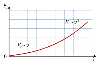
Зависимость силы от сопротивления определяется для каждой среды отдельно. Сила сопротивления среды растет, с ростом скорости движения предмета в среде.
От чего зависит сила сопротивления
На величину силы сопротивления влияют следующие факторы:
- особенности и плотность среды, например, у жидкости плотность выше, чем у газа;
- форма тела, у предметов с вытянутыми обтекаемыми вдоль движения формами сопротивление меньше, чем с расположенными перпендикулярно движению гранями;
- скорость движения.
В зависимости от воздействия на движущиеся предметы различают несколько типов силы сопротивления:
- Сила сопротивления качению [P_{f}]. Зависит от вида и состояния опорной поверхности, скорости перемещения, силы давления воздуха и прочее. Коэффициент сопротивлению качению f зависит типа и состояния опорной поверхности, его значение уменьшается, при повышении давления и температуры.
- Сила сопротивления воздуха [P_{B}] возникает при разных показателях давления. В аэродинамике называется лобовым сопротивлением. Показатель будет выше с ростом вихреобразования в передней и задней частях объекта движения. Величина вихреобразования зависит от формы передвигаемых предметов.
Понятие силы электрического сопротивления
Строение металлических проводников объясняет наличие сопротивления. Свободные электроны движутся по проводнику встречая ионы кристаллической решетки. При контакте с ними другие электроны теряют часть своей энергии. У проводников с отличающимся атомным строением будет разное сопротивление току. Поэтому чем выше сопротивление проводника, тем проводимость электрического тока будет меньше.

Формулы 4 — 5
Электрическое сопротивление в физике обозначают R, измеряется в Ом. Сопротивление равно 1 Ом, если на концах проводника возникает напряжение в 1 Вольт при силе тока равной 1 Ампер.
Формула сопротивления силы тока:
[R=rho frac{l}{S}]
где l – длина проводника; S – площадь сечения; ρ – удельное сопротивление.
Сила электрического сопротивления зависит от материала проводника, его длины, формы и температуры. Удельное сопротивление отличается у различных материалов.
Удельное сопротивление [boldsymbol{(rho)}] — сопротивление проводника длиной 1м и обладающего площадью поперечного сечения [boldsymbol{1м^{2}}]. Обозначается в Ом*м. К примеру, удельное сопротивления меди [1,7 * 10^{-8} Oм * м], это значит, что у медного проводника длиной [1м^{2}] сопротивление равно [1,7 * 10^{-8} Ом].
Сопротивление проводника будет расти с увеличением температуры:
[rho=rho_{o}(1+alpha Delta T)]
где [boldsymbol{rho_{0}}] – обозначает удельное сопротивление при [T_{0}=293 mathrm{~K}left(20^{circ} mathrm{C}right), Delta T=T-T_{0}], α – температурный коэффициент сопротивления [left(K^{-1}right)].
При нагревании движение частиц материала возрастает и создает препятствия для направленного движения электродов. Количество столкновений свободных электронов с ионами кристаллической решетки увеличивается.
Такое свойство применимо в термометрах сопротивления, измеряют температуру исходя из зависимости температуры и сопротивления с высокой точностью измерения.

Нет времени решать самому?
Наши эксперты помогут!
Формула силы тока и сопротивление
Формула 6
Законом Ома для участка цепи называют взаимосвязь между силой тока (I), напряжением (U) и сопротивлением (R) проводника на практике установлена Г. Омом.
[I=frac{U}{R}]
Материалы с низким удельным сопротивлением считаются проводниками, они эффективно проводят электрический ток. С высоким удельным сопротивлением – диэлектрики, их используют как изоляторы. Промежуточное положение занимают полупроводники.
Пример
Найти силу тока в проводнике длиной 100 мм, сечением 0,5 мм2 изготовленном из меди, если напряжение на его концах 6,8 В.
Решение:
Запишем формулу закона Ома и найдем сопротивление через силу тока : [I=frac{U}{R}]
Для определения силы тока I, нужно определить сопротивление R. С помощью формулы с удельным сопротивлением преобразуем формулу для закона Ома:
[begin{array}{r}
R=rho frac{l}{S} \
I=frac{U S}{rho l}
end{array}]
Подставляем значения в формулу:
[I=frac{6,8 * 0,5}{0,017 * 100}=2 mathrm{~A}]
Значение ρ для меди берется из таблиц.
Ответ: 2А

Виктор Матвеевич Скоков
Эксперт по предмету «Физика»
Задать вопрос автору статьи
При совершенно любом движении будет фиксироваться появление между поверхностями тел или в среде, где оно осуществляется, сил сопротивления. Второе свойственное им название – силы трения.
Замечание 1
Силы сопротивления могут быть зависимыми от разновидностей трущихся поверхностей, реакций опоры тела, а также его скорости, при условии движения тела в вязкой среде (к примеру, в воздухе или воде).
Расчет сил сопротивления
С целью определения сил сопротивления потребуется применение третьего закона Ньютона. Такая величина, как сила сопротивления, будет численно равной силе, которую потребуется приложить с целью равномерного движения предмета по горизонтальной ровной поверхности. Это становится возможным с помощью динамометра.
Таким образом, искомая величина оказывается прямо пропорциональной массе тела. Стоит при этом учитывать во внимание, что для более точного подсчета потребуется выбрать $u$ коэффициент, зависимый от материала изготовления опоры. Также принимается во внимание материал изготовления самого предмета исследования. При расчете применяется постоянная $g$, чье значение 9,8 $м/с^2$.
В условиях движения тела на высоте, на него влияет сила трения воздуха, зависимая от скорости перемещения предмета. Искомую величину определяют на основании такой формулы (подходящей исключительно для тел с передвижением с небольшой скоростью):
$F = va$, где:
- $v$ – скорость движения предмета,
- $a$ – коэффициент сопротивления среды.
Разновидности сил сопротивления
Существуют такие разновидности сил сопротивления:
- Сила сопротивления качению $P_f$, зависимая от таких факторов, как: разновидности и состояния опорной поверхности, скорости движения, давления воздуха и пр. Коэффициент сопротивления качению $f$ зависеть при этом состояния и типа опорной поверхности. С повышением температуры и давления, указанный коэффициент уменьшается.
- Сила сопротивления воздуха (лобовое сопротивление) $Р_в$ возникает за счет разницы давлений. Данный показатель окажется тем выше, чем большим будет вихреобразование как в передней, так и в задней части объекта движения. Величина вихреобразования будет зависеть от формы движущихся тел.
«Силы сопротивления» 👇
Наиболее значимым будет воздействие на сопротивление движению передней части. Так, при создании закругления в передней и задней части плоскостенной фигуры, сопротивление возможно уменьшить на 72 %. Сила лобового сопротивления $Р_{вл}$ определяется по такой формуле:
$P_{вл} = {c_xpF_в}frac{v^2}{2}$, где:
- $с_х$– коэффициент лобового сопротивления (обтекаемости);
- $p$- плотность воздуха;
- $F_в$ –площадь лобового сопротивления (миделевого сечения) определяется по формуле
Сила сопротивления воздуха ориентирована в направлении, противоположном вектору скорости объекта движения (например, автомобиля). Обычно она рассматривается как сконцентрированная сила, приложенная в отношении точки (центра парусности объекта), не совпадающей при этом с центром массы исследуемого объекта.
Сила сопротивления разгону поступательно движущейся массы объекта, согласно второму закону Ньютона, определяется таким образом:
$Рj = mfrac{dV}{dt}$, где:
- $m$– масса автомобиля;
- $frac{dv}{dt}$ — ускорение центра масс.
Силы сопротивления при больших скоростях
В случае, когда мы имеем дело с малыми скоростями, сопротивление будет зависеть от:
- вязкости жидкости;
- скорости движения;
- линейных размеров тела.
Рассмотрим действие законов трения при больших скоростях. Так, к воздуху и в особенности, к воде законы вязкого трения будут мало применимыми. Даже при наличии таких скоростей, как 1 см/с, они будут пригодными исключительно в отношении тел крошечных размеров (в миллиметрах).
Замечание 2
Сопротивление, которое испытывает ныряющий в воду пловец, ни в коей мере не будет подчиняться действию закона вязкого трения.
При медленном движении жидкость станет плавно обтекать предмет движения. При этом сила сопротивления, которую он будет преодолевать, и окажется силой вязкого трения.
В условиях большой скорости, позади движущегося объекта возникнет уже более сложное движение жидкости. В жидкости начнут то появляться, то исчезать разные струйки, формируя при этом необычные по форме фигуры, вихри, кольца. Таким образом, картина струек будет подвержена постоянным изменениям. Возникновение подобного движения получило название турбулентного.
Турбулентное сопротивление будет зависимым от скорости и размеров предмета не так, как при вязком. Так, оно окажется пропорциональным квадратам скорости и линейных размеров. Вязкость жидкости при подобном движении перестает иметь решающее значение, а определяющим свойством выступает ее плотность. Таким образом, для силы $F$ турбулентного сопротивления справедлива формула:
$F=pv^2L^2$, где:
- $v$– скорость движения,
- $L$– линейные размеры предмета,
- $p$ – плотность среды.
Находи статьи и создавай свой список литературы по ГОСТу
Поиск по теме
For other uses, see Drag.
In fluid dynamics, drag (sometimes called air resistance, a type of friction, or fluid resistance, another type of friction or fluid friction) is a force acting opposite to the relative motion of any object moving with respect to a surrounding fluid.[1] This can exist between two fluid layers (or surfaces) or between a fluid and a solid surface. Unlike other resistive forces, such as dry friction, which are nearly independent of velocity, the drag force depends on velocity.[2][3]
Drag force is proportional to the velocity for low-speed flow and the squared velocity for high speed flow, where the distinction between low and high speed is measured by the Reynolds number. Even though the ultimate cause of drag is viscous friction, turbulent drag is independent of viscosity.[4]
Drag forces always tend to decrease fluid velocity relative to the solid object in the fluid’s path.
Examples[edit]
Examples of drag include the component of the net aerodynamic or hydrodynamic force acting opposite to the direction of movement of a solid object such as cars (automobile drag coefficient), aircraft[3] and boat hulls; or acting in the same geographical direction of motion as the solid, as for sails attached to a down wind sail boat, or in intermediate directions on a sail depending on points of sail.[5][6][7] In the case of viscous drag of fluid in a pipe, drag force on the immobile pipe decreases fluid velocity relative to the pipe.[8][9]
In the physics of sports, the drag force is necessary to explain the motion of balls, javelins, arrows and frisbees and the performance of runners and swimmers.[10]
Types[edit]
| Shape and flow | Form Drag |
Skin friction |
|---|---|---|
| ≈0% | ≈100% | |
| ≈10% | ≈90% | |

|
≈90% | ≈10% |

|
≈100% | ≈0% |
Types of drag are generally divided into the following categories:
- form drag or pressure drag due to the size and shape of a body
- skin friction drag or viscous drag due to the friction between the fluid and a surface which may be the outside of an object or inside such as the bore of a pipe
The effect of streamlining on the relative proportions of skin friction and form drag is shown for two different body sections, an airfoil, which is a streamlined body, and a cylinder, which is a bluff body. Also shown is a flat plate illustrating the effect that orientation has on the relative proportions of skin friction and pressure difference between front and back. A body is known as bluff (or blunt) if the source of drag is dominated by pressure forces and streamlined if the drag is dominated by viscous forces. Road vehicles are bluff bodies.[11] For aircraft, pressure and friction drag are included in the definition of parasitic drag. Parasite drag is often expressed in terms of a hypothetical (in so far as there is no edge spillage drag[12]) «equivalent parasite drag area» which is the area of a flat plate perpendicular to the flow. It is used for comparing the drag of different aircraft. For example, the Douglas DC-3 has an equivalent parasite area of 23.7 sq ft and the McDonnell Douglas DC-9, with 30 years of advancement in aircraft design, an area of 20.6 sq ft although it carried five times as many passengers.[13]
- lift-induced drag appears with wings or a lifting body in aviation and with semi-planing or planing hulls for watercraft
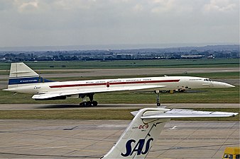
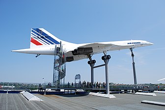
- wave drag (aerodynamics) is caused by the presence of shockwaves and first appears at subsonic aircraft speeds when local flow velocities become supersonic. The wave drag of the supersonic Concorde prototype aircraft was reduced at Mach 2 by 1.8% by applying the area rule which extended the rear fuselage 3.73m on the production aircraft.[14]
- wave resistance (ship hydrodynamics) or wave drag occurs when a solid object is moving along a fluid boundary and making surface waves
- boat-tail drag on an aircraft is caused by the angle with which the rear fuselage, or engine nacelle, narrows to the engine exhaust diameter.[15]
-

Concorde with ‘high’ wave drag tail
-

Concorde with ‘low’ wave drag tail
-

Hawk aircraft showing base area above circular engine exhaust

The drag equation[edit]

Drag coefficient Cd for a sphere as a function of Reynolds number Re, as obtained from laboratory experiments. The dark line is for a sphere with a smooth surface, while the lighter line is for the case of a rough surface.
Drag depends on the properties of the fluid and on the size, shape, and speed of the object. One way to express this is by means of the drag equation:

where
 is the drag force,
- is the density of the fluid,[16]
- is the speed of the object relative to the fluid,
- is the cross sectional area, and
- is the drag coefficient – a dimensionless number.


The drag coefficient depends on the shape of the object and on the Reynolds number
- ,

where
- is some characteristic diameter or linear dimension. Actually it is the equivalent diameter of the object. For a sphere is the D of the sphere itself.
- For a rectangular shape cross-section in the motion direction, , where a and b are the rectangle edges.
- is the kinematic viscosity of the fluid (equal to the dynamic viscosity divided by the density ).


At low  ,
,  is asymptotically proportional to
  , which means that the drag is linearly proportional to the speed, i.e. the drag force on a small sphere moving through a viscous fluid is given by the Stokes Law:

At high , is more or less constant and drag will vary as the square of the speed. The graph to the right shows how varies with for the case of a sphere. Since the power needed to overcome the drag force is the product of the force times speed, the power needed to overcome drag will vary as the square of the speed at low Reynolds numbers and as the cube of the speed at high numbers.
It can be demonstrated that drag force can be expressed as a function of a dimensionless number, which is dimensionally identical to the Bejan number.[17] Consequently, drag force and drag coefficient can be a function of Bejan number. In fact, from the expression of drag force it has been obtained:

and consequently allows expressing the drag coefficient as a function of Bejan number and the ratio between wet area  and front area
  :[17]
:[17]

where  is the Reynolds number related to fluid path length L.
At high velocity[edit]
Explanation of drag by NASA.
As mentioned, the drag equation with a constant drag coefficient gives the force experienced by an object moving through a fluid at relatively large velocity (i.e. high Reynolds number, Re > ~1000). This is also called quadratic drag. The equation is attributed to Lord Rayleigh, who originally used L2 in place of A (L being some length).

see derivation
The reference area A is often orthographic projection of the object (frontal area)—on a plane perpendicular to the direction of motion—e.g. for objects with a simple shape, such as a sphere, this is the cross sectional area. Sometimes a body is a composite of different parts, each with a different reference areas, in which case a drag coefficient corresponding to each of those different areas must be determined.
In the case of a wing the reference areas are the same and the drag force is in the same ratio to the lift force as the ratio of drag coefficient to lift coefficient.[18] Therefore, the reference for a wing is often the lifting area («wing area») rather than the frontal area.[19]
For an object with a smooth surface, and non-fixed separation points—like a sphere or circular cylinder—the drag coefficient may vary with Reynolds number Re, even up to very high values (Re of the order 107).
[20]
[21]
For an object with well-defined fixed separation points, like a circular disk with its plane normal to the flow direction, the drag coefficient is constant for Re > 3,500.[21]
Further the drag coefficient Cd is, in general, a function of the orientation of the flow with respect to the object (apart from symmetrical objects like a sphere).
Power[edit]
Under the assumption that the fluid is not moving relative to the currently used reference system, the power required to overcome the aerodynamic drag is given by:

Note that the power needed to push an object through a fluid increases as the cube of the velocity. A car cruising on a highway at 50 mph (80 km/h) may require only 10 horsepower (7.5 kW) to overcome aerodynamic drag, but that same car at 100 mph (160 km/h) requires 80 hp (60 kW).[22] With a doubling of speed the drag (force) quadruples per the formula. Exerting 4 times the force over a fixed distance produces 4 times as much work. At twice the speed the work (resulting in displacement over a fixed distance) is done twice as fast. Since power is the rate of doing work, 4 times the work done in half the time requires 8 times the power.
When the fluid is moving relative to the reference system (e.g. a car driving into headwind) the power required to overcome the aerodynamic drag is given by:

Where  is the wind speed and
  is the object speed (both relative to ground).
Velocity of a falling object[edit]

An object falling through viscous medium accelerates quickly towards its terminal speed, approaching gradually as the speed gets nearer to the terminal speed. Whether the object experiences turbulent or laminar drag changes the characteristic shape of the graph with turbulent flow resulting in a constant acceleration for a larger fraction of its accelerating time.
The velocity as a function of time for an object falling through a non-dense medium, and released at zero relative-velocity v = 0 at time t = 0, is roughly given by a function involving a hyperbolic tangent (tanh):

The hyperbolic tangent has a limit value of one, for large time t. In other words, velocity asymptotically approaches a maximum value called the terminal velocity vt:

For an object falling and released at relative-velocity v = vi at time t = 0, with vi < vt, is also defined in terms of the hyperbolic tangent function:

For vi > vt, the velocity function is defined in terms of the hyperbolic cotangent function:

The hyperbolic cotangent has also a limit value of one, for large time t. Velocity asymptotically tends to the terminal velocity vt, strictly from above vt.
For vi = vt, the velocity is constant:

Actually, these functions are defined by the solution of the following differential equation:

Or, more generically (where F(v) are the forces acting on the object beyond drag):

For a potato-shaped object of average diameter d and of density ρobj, terminal velocity is about

For objects of water-like density (raindrops, hail, live objects—mammals, birds, insects, etc.) falling in air near Earth’s surface at sea level, the terminal velocity is roughly equal to

with d in metre and vt in m/s. For example, for a human body ( ≈0.6 m)
  ≈70 m/s, for a small animal like a cat ( ≈0.2 m) ≈40 m/s, for a small bird ( ≈0.05 m) ≈20 m/s, for an insect ( ≈0.01 m) ≈9 m/s, and so on. Terminal velocity for very small objects (pollen, etc.) at low Reynolds numbers is determined by Stokes law.
Terminal velocity is higher for larger creatures, and thus potentially more deadly. A creature such as a mouse falling at its terminal velocity is much more likely to survive impact with the ground than a human falling at its terminal velocity. A small animal such as a cricket impacting at its terminal velocity will probably be unharmed. This, combined with the relative ratio of limb cross-sectional area vs. body mass (commonly referred to as the square–cube law), explains why very small animals can fall from a large height and not be harmed.[23]
Very low Reynolds numbers: Stokes’ drag[edit]
Trajectories of three objects thrown at the same angle (70°). The black object does not experience any form of drag and moves along a parabola. The blue object experiences Stokes’ drag, and the green object Newton drag.
The equation for viscous resistance or linear drag is appropriate for objects or particles moving through a fluid at relatively slow speeds where there is no turbulence (i.e. low Reynolds number,  ).[24] Note that purely laminar flow only exists up to Re = 0.1 under this definition. In this case, the force of drag is approximately proportional to velocity. The equation for viscous resistance is:[25]

where:
- is a constant that depends on both the material properties of the object and fluid, as well as the geometry of the object; and
- is the velocity of the object.

When an object falls from rest, its velocity will be

where:
- is the density of the object,
- is density of the fluid,
- is the volume of the object,
- is the acceleration due to gravity (i.e., 9.8 m/s), and
- is mass of the object.


The velocity asymptotically approaches the terminal velocity  . For a given
  , denser objects fall more quickly.
For the special case of small spherical objects moving slowly through a viscous fluid (and thus at small Reynolds number), George Gabriel Stokes derived an expression for the drag constant:

where:
- is the Stokes radius of the particle, and is the fluid viscosity.

The resulting expression for the drag is known as Stokes’ drag:[26]

For example, consider a small sphere with radius  = 0.5 micrometre (diameter = 1.0 µm) moving through water at a velocity
  of 10 µm/s. Using 10−3 Pa·s as the dynamic viscosity of water in SI units,
we find a drag force of 0.09 pN. This is about the drag force that a bacterium experiences as it swims through water.
The drag coefficient of a sphere can be determined for the general case of a laminar flow with Reynolds numbers less than 1 using the following formula:[27]

For Reynolds numbers less than 1, Stokes’ law applies and the drag coefficient approaches  !
!
Aerodynamics[edit]
In aerodynamics, aerodynamic drag is the fluid drag force that acts on any moving solid body in the direction of the fluid freestream flow.[28] From the body’s perspective (near-field approach), the drag results from forces due to pressure distributions over the body surface, symbolized  , and forces due to skin friction, which is a result of viscosity, denoted
  . Alternatively, calculated from the flowfield perspective (far-field approach), the drag force results from three natural phenomena: shock waves, vortex sheet, and viscosity.
Overview[edit]
The pressure distribution acting on a body’s surface exerts normal forces on the body. Those forces can be summed and the component of that force that acts downstream represents the drag force, , due to pressure distribution acting on the body. The nature of these normal forces combines shock wave effects, vortex system generation effects, and wake viscous mechanisms.
The viscosity of the fluid has a major effect on drag. In the absence of viscosity, the pressure forces acting to retard the vehicle are canceled by a pressure force further aft that acts to push the vehicle forward; this is called pressure recovery and the result is that the drag is zero. That is to say, the work the body does on the airflow, is reversible and is recovered as there are no frictional effects to convert the flow energy into heat. Pressure recovery acts even in the case of viscous flow. Viscosity, however results in pressure drag and it is the dominant component of drag in the case of vehicles with regions of separated flow, in which the pressure recovery is fairly ineffective.
The friction drag force, which is a tangential force on the aircraft surface, depends substantially on boundary layer configuration and viscosity. The net friction drag, , is calculated as the downstream projection of the viscous forces evaluated over the body’s surface.
The sum of friction drag and pressure (form) drag is called viscous drag. This drag component is due to viscosity. In a thermodynamic perspective, viscous effects represent irreversible phenomena and, therefore, they create entropy. The calculated viscous drag  use entropy changes to accurately predict the drag force.
When the airplane produces lift, another drag component results. Induced drag, symbolized  , is due to a modification of the pressure distribution due to the trailing vortex system that accompanies the lift production. An alternative perspective on lift and drag is gained from considering the change of momentum of the airflow. The wing intercepts the airflow and forces the flow to move downward. This results in an equal and opposite force acting upward on the wing which is the lift force. The change of momentum of the airflow downward results in a reduction of the rearward momentum of the flow which is the result of a force acting forward on the airflow and applied by the wing to the air flow; an equal but opposite force acts on the wing rearward which is the induced drag. Another drag component, namely wave drag,
  , results from shock waves in transonic and supersonic flight speeds. The shock waves induce changes in the boundary layer and pressure distribution over the body surface.
In summary, there are three ways of categorising drag.[29]: 19
- Pressure drag and friction drag
- Profile drag and induced drag
- Vortex drag, wave drag and wake drag
History[edit]
The idea that a moving body passing through air or another fluid encounters resistance had been known since the time of Aristotle. According to Mervyn O’Gorman, this was named «drag» by Archibald Reith Low.[30] Louis Charles Breguet’s paper of 1922 began efforts to reduce drag by streamlining.[31] Breguet went on to put his ideas into practice by designing several record-breaking aircraft in the 1920s and 1930s. Ludwig Prandtl’s boundary layer theory in the 1920s provided the impetus to minimise skin friction. A further major call for streamlining was made by Sir Melvill Jones who provided the theoretical concepts to demonstrate emphatically the importance of streamlining in aircraft design.[32][33][34]
In 1929 his paper ‘The Streamline Airplane’ presented to the Royal Aeronautical Society was seminal. He proposed an ideal aircraft that would have minimal drag which led to the concepts of a ‘clean’ monoplane and retractable undercarriage. The aspect of Jones’s paper that most shocked the designers of the time was his plot of the horse power required versus velocity, for an actual and an ideal plane. By looking at a data point for a given aircraft and extrapolating it horizontally to the ideal curve, the velocity gain for the same power can be seen. When Jones finished his presentation, a member of the audience described the results as being of the same level of importance as the Carnot cycle in thermodynamics.[31][32]
Lift-induced drag and parasitic drag[edit]
Lift-induced drag[edit]
Lift-induced drag (also called induced drag) is drag which occurs as the result of the creation of lift on a three-dimensional lifting body, such as the wing or fuselage of an airplane. Induced drag consists primarily of two components: drag due to the creation of trailing vortices (vortex drag); and the presence of additional viscous drag (lift-induced viscous drag) that is not present when lift is zero. The trailing vortices in the flow-field, present in the wake of a lifting body, derive from the turbulent mixing of air from above and below the body which flows in slightly different directions as a consequence of creation of lift.
With other parameters remaining the same, as the lift generated by a body increases, so does the lift-induced drag. This means that as the wing’s angle of attack increases (up to a maximum called the stalling angle), the lift coefficient also increases, and so too does the lift-induced drag. At the onset of stall, lift is abruptly decreased, as is lift-induced drag, but viscous pressure drag, a component of parasite drag, increases due to the formation of turbulent unattached flow in the wake behind the body.
Parasitic drag[edit]
Parasitic drag, or profile drag, is drag caused by moving a solid object through a fluid. Parasitic drag is made up of multiple components including viscous pressure drag (form drag), and drag due to surface roughness (skin friction drag). Additionally, the presence of multiple bodies in relative proximity may incur so called interference drag, which is sometimes described as a component of parasitic drag.
In aviation, induced drag tends to be greater at lower speeds because a high angle of attack is required to maintain lift, creating more drag. However, as speed increases the angle of attack can be reduced and the induced drag decreases. Parasitic drag, however, increases because the fluid is flowing more quickly around protruding objects increasing friction or drag. At even higher speeds (transonic), wave drag enters the picture. Each of these forms of drag changes in proportion to the others based on speed. The combined overall drag curve therefore shows a minimum at some airspeed — an aircraft flying at this speed will be at or close to its optimal efficiency. Pilots will use this speed to maximize endurance (minimum fuel consumption), or maximize gliding range in the event of an engine failure.
Power curve in aviation[edit]
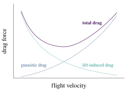
The power curve: parasitic drag and lift-induced drag vs. airspeed
The interaction of parasitic and induced drag vs. airspeed can be plotted as a characteristic curve, illustrated here. In aviation, this is often referred to as the power curve, and is important to pilots because it shows that, below a certain airspeed, maintaining airspeed counterintuitively requires more thrust as speed decreases, rather than less. The consequences of being «behind the curve» in flight are important and are taught as part of pilot training. At the subsonic airspeeds where the «U» shape of this curve is significant, wave drag has not yet become a factor, and so it is not shown in the curve.
Wave drag in transonic and supersonic flow[edit]

Qualitative variation in Cd factor with Mach number for aircraft
Wave drag (also called compressibility drag) is drag that is created when a body moves in a compressible fluid and at speeds that are close to the speed of sound in that fluid. In aerodynamics, wave drag consists of multiple components depending on the speed regime of the flight.
In transonic flight (Mach numbers greater than about 0.8 and less than about 1.4), wave drag is the result of the formation of shockwaves in the fluid, formed when local areas of supersonic (Mach number greater than 1.0) flow are created. In practice, supersonic flow occurs on bodies traveling well below the speed of sound, as the local speed of air increases as it accelerates over the body to speeds above Mach 1.0. However, full supersonic flow over the vehicle will not develop until well past Mach 1.0. Aircraft flying at transonic speed often incur wave drag through the normal course of operation. In transonic flight, wave drag is commonly referred to as transonic compressibility drag. Transonic compressibility drag increases significantly as the speed of flight increases towards Mach 1.0, dominating other forms of drag at those speeds.
In supersonic flight (Mach numbers greater than 1.0), wave drag is the result of shockwaves present in the fluid and attached to the body, typically oblique shockwaves formed at the leading and trailing edges of the body. In highly supersonic flows, or in bodies with turning angles sufficiently large, unattached shockwaves, or bow waves will instead form. Additionally, local areas of transonic flow behind the initial shockwave may occur at lower supersonic speeds, and can lead to the development of additional, smaller shockwaves present on the surfaces of other lifting bodies, similar to those found in transonic flows. In supersonic flow regimes, wave drag is commonly separated into two components, supersonic lift-dependent wave drag and supersonic volume-dependent wave drag.
The closed form solution for the minimum wave drag of a body of revolution with a fixed length was found by Sears and Haack, and is known as the Sears-Haack Distribution. Similarly, for a fixed volume, the shape for minimum wave drag is the Von Karman Ogive.
The Busemann biplane theoretical concept is not subject to wave drag when operated at its design speed, but is incapable of generating lift in this condition.
d’Alembert’s paradox[edit]
In 1752 d’Alembert proved that potential flow, the 18th century state-of-the-art inviscid flow theory amenable to mathematical solutions, resulted in the prediction of zero drag. This was in contradiction with experimental evidence, and became known as d’Alembert’s paradox. In the 19th century the Navier–Stokes equations for the description of viscous flow were developed by Saint-Venant, Navier and Stokes. Stokes derived the drag around a sphere at very low Reynolds numbers, the result of which is called Stokes’ law.[35]
In the limit of high Reynolds numbers, the Navier–Stokes equations approach the inviscid Euler equations, of which the potential-flow solutions considered by d’Alembert are solutions. However, all experiments at high Reynolds numbers showed there is drag. Attempts to construct inviscid steady flow solutions to the Euler equations, other than the potential flow solutions, did not result in realistic results.[35]
The notion of boundary layers—introduced by Prandtl in 1904, founded on both theory and experiments—explained the causes of drag at high Reynolds numbers. The boundary layer is the thin layer of fluid close to the object’s boundary, where viscous effects remain important even when the viscosity is very small (or equivalently the Reynolds number is very large).[35]
See also[edit]
- Added mass
- Aerodynamic force
- Angle of attack
- Atmospheric density
- Automobile drag coefficient
- Boundary layer
- Coandă effect
- Drag crisis
- Drag coefficient
- Drag equation
- Gravity drag
- Keulegan–Carpenter number
- Lift (force)
- Morison equation
- Nose cone design
- Parasitic drag
- Projectile motion#Trajectory of a projectile with air resistance
- Ram pressure
- Reynolds number
- Stall (fluid mechanics)
- Stokes’ law
- Terminal velocity
- Wave drag
- Windage
References[edit]
- ^ «Definition of DRAG». www.merriam-webster.com.
- ^ French (1970), p. 211, Eq. 7-20
- ^ a b «What is Drag?». Archived from the original on 2010-05-24. Retrieved 2011-10-16.
- ^ G. Falkovich (2011). Fluid Mechanics (A short course for physicists). Cambridge University Press. ISBN 978-1-107-00575-4.
- ^ Eiffel, Gustave (1913). The Resistance of The Air and Aviation. London: Constable &Co Ltd.
- ^ Marchaj, C. A. (2003). Sail performance : techniques to maximise sail power (Rev. ed.). London: Adlard Coles Nautical. pp. 147 figure 127 lift vs drag polar curves. ISBN 978-0-7136-6407-2.
- ^ Drayton, Fabio Fossati; translated by Martyn (2009). Aero-hydrodynamics and the performance of sailing yachts : the science behind sailing yachts and their design. Camden, Maine: International Marine /McGraw-Hill. pp. 98 Fig 5.17 Chapter five Sailing Boat Aerodynamics. ISBN 978-0-07-162910-2.
- ^ «Calculating Viscous Flow: Velocity Profiles in Rivers and Pipes» (PDF). Retrieved 16 October 2011.
- ^ «Viscous Drag Forces». Retrieved 16 October 2011.
- ^ Hernandez-Gomez, J J; Marquina, V; Gomez, R W (25 July 2013). «On the performance of Usain Bolt in the 100 m sprint». Eur. J. Phys. 34 (5): 1227–1233. arXiv:1305.3947. Bibcode:2013EJPh…34.1227H. doi:10.1088/0143-0807/34/5/1227. S2CID 118693492. Retrieved 23 April 2016.
- ^ Encyclopedia of Automotive Engineering, David Crolla, Paper «Fundamentals, Basic principles in Road vehicle Aerodynamics and Design», ISBN 978 0 470 97402 5
- ^ The Design Of The Aeroplane, Darrol Stinton, ISBN 0 632 01877 1, p.204
- ^ Fundamentals of Flight, Second Edition, Richard S. Shevell,ISBN 0 13 339060 8, p.185
- ^ A Case Study By Aerospatiale And British Aerospace On The Concorde By Jean Rech and Clive S. Leyman,AIAA Professional Study Series, Fig. 3.6
- ^ Design For Air Combat, Ray Whitford,ISBN 0 7106 0426 2, p.212
- ^ Note that for Earth’s atmosphere, the air density can be found using the barometric formula. It is 1.293 kg/m3 at 0 °C and 1 atmosphere.
- ^ a b Liversage, P., and Trancossi, M. (2018). Analysis of triangular sharkskin profiles according to second law, Modelling, Measurement and Control B. 87(3), 188-196. http://www.iieta.org/sites/default/files/Journals/MMC/MMC_B/87.03_11.pdf
- ^ Size effects on drag Archived 2016-11-09 at the Wayback Machine, from NASA Glenn Research Center.
- ^ Wing geometry definitions Archived 2011-03-07 at the Wayback Machine, from NASA Glenn Research Center.
- ^ Roshko, Anatol (1961). «Experiments on the flow past a circular cylinder at very high Reynolds number» (PDF). Journal of Fluid Mechanics. 10 (3): 345–356. Bibcode:1961JFM….10..345R. doi:10.1017/S0022112061000950. S2CID 11816281.
- ^ a b Batchelor (1967), p. 341.
- ^ Brian Beckman (1991), Part 6: Speed and Horsepower, archived from the original on 2016-06-16, retrieved 18 May 2016
- ^ Haldane, J.B.S., «On Being the Right Size» Archived 2011-08-22 at the Wayback Machine
- ^ Drag Force Archived April 14, 2008, at the Wayback Machine
- ^ Air friction, from Department of Physics and Astronomy, Georgia State University
- ^ Collinson, Chris; Roper, Tom (1995). Particle Mechanics. Butterworth-Heinemann. p. 30. ISBN 9780080928593.
- ^ tec-science (2020-05-31). «Drag coefficient (friction and pressure drag)». tec-science. Retrieved 2020-06-25.
- ^ Anderson, John D. Jr., Introduction to Flight
- ^ Gowree, Erwin Ricky (20 May 2014). Influence of Attachment Line Flow on Form Drag (doctoral). Retrieved 22 March 2022.
- ^ https://archive.org/details/Flight_International_Magazine_1913-02-01-pdf/page/n19/mode/2up Flight, 1913, p. 126
- ^ a b Anderson, John David (1929). A History of Aerodynamics: And Its Impact On Flying Machines. University of Cambridge.
- ^ a b «University of Cambridge Engineering Department». Retrieved 28 Jan 2014.
- ^ Sir Morien Morgan, Sir Arnold Hall (November 1977). Biographical Memoirs of Fellows of the Royal Society Bennett Melvill Jones. 28 January 1887 — 31 October 1975. Vol. 23. The Royal Society. pp. 252–282.
- ^ Mair, W.A. (1976). Oxford Dictionary of National Biography.
- ^ a b c Batchelor (2000), pp. 337–343.
- ‘Improved Empirical Model for Base Drag Prediction on Missile Configurations, based on New Wind Tunnel Data’, Frank G Moore et al. NASA Langley Center
- ‘Computational Investigation of Base Drag Reduction for a Projectile at Different Flight Regimes’, M A Suliman et al. Proceedings of 13th International Conference on Aerospace Sciences & Aviation Technology, ASAT- 13, May 26 – 28, 2009
- ‘Base Drag and Thick Trailing Edges’, Sighard F. Hoerner, Air Materiel Command, in: Journal of the Aeronautical Sciences, Oct 1950, pp 622–628
Bibliography[edit]
- French, A. P. (1970). Newtonian Mechanics (The M.I.T. Introductory Physics Series) (1st ed.). W. W. Norton & Company Inc., New York. ISBN 978-0-393-09958-4.
- G. Falkovich (2011). Fluid Mechanics (A short course for physicists). Cambridge University Press. ISBN 978-1-107-00575-4.
- Serway, Raymond A.; Jewett, John W. (2004). Physics for Scientists and Engineers (6th ed.). Brooks/Cole. ISBN 978-0-534-40842-8.
- Tipler, Paul (2004). Physics for Scientists and Engineers: Mechanics, Oscillations and Waves, Thermodynamics (5th ed.). W. H. Freeman. ISBN 978-0-7167-0809-4.
- Huntley, H. E. (1967). Dimensional Analysis. Dover. LOC 67-17978.
- Batchelor, George (2000). An introduction to fluid dynamics. Cambridge Mathematical Library (2nd ed.). Cambridge University Press. ISBN 978-0-521-66396-0. MR 1744638.
- L. J. Clancy (1975), Aerodynamics, Pitman Publishing Limited, London. ISBN 978-0-273-01120-0
- Anderson, John D. Jr. (2000); Introduction to Flight, Fourth Edition, McGraw Hill Higher Education, Boston, Massachusetts, USA. 8th ed. 2015, ISBN 978-0078027673.
External links[edit]
- Educational materials on air resistance
- Aerodynamic Drag and its effect on the acceleration and top speed of a vehicle.
- Vehicle Aerodynamic Drag calculator based on drag coefficient, frontal area and speed.
- Smithsonian National Air and Space Museum’s How Things Fly website
- Effect of dimples on a golf ball and a car
For other uses, see Drag.
In fluid dynamics, drag (sometimes called air resistance, a type of friction, or fluid resistance, another type of friction or fluid friction) is a force acting opposite to the relative motion of any object moving with respect to a surrounding fluid.[1] This can exist between two fluid layers (or surfaces) or between a fluid and a solid surface. Unlike other resistive forces, such as dry friction, which are nearly independent of velocity, the drag force depends on velocity.[2][3]
Drag force is proportional to the velocity for low-speed flow and the squared velocity for high speed flow, where the distinction between low and high speed is measured by the Reynolds number. Even though the ultimate cause of drag is viscous friction, turbulent drag is independent of viscosity.[4]
Drag forces always tend to decrease fluid velocity relative to the solid object in the fluid’s path.
Examples[edit]
Examples of drag include the component of the net aerodynamic or hydrodynamic force acting opposite to the direction of movement of a solid object such as cars (automobile drag coefficient), aircraft[3] and boat hulls; or acting in the same geographical direction of motion as the solid, as for sails attached to a down wind sail boat, or in intermediate directions on a sail depending on points of sail.[5][6][7] In the case of viscous drag of fluid in a pipe, drag force on the immobile pipe decreases fluid velocity relative to the pipe.[8][9]
In the physics of sports, the drag force is necessary to explain the motion of balls, javelins, arrows and frisbees and the performance of runners and swimmers.[10]
Types[edit]
| Shape and flow | Form Drag |
Skin friction |
|---|---|---|
| ≈0% | ≈100% | |
| ≈10% | ≈90% | |
|
|
≈90% | ≈10% |
|
|
≈100% | ≈0% |
Types of drag are generally divided into the following categories:
- form drag or pressure drag due to the size and shape of a body
- skin friction drag or viscous drag due to the friction between the fluid and a surface which may be the outside of an object or inside such as the bore of a pipe
The effect of streamlining on the relative proportions of skin friction and form drag is shown for two different body sections, an airfoil, which is a streamlined body, and a cylinder, which is a bluff body. Also shown is a flat plate illustrating the effect that orientation has on the relative proportions of skin friction and pressure difference between front and back. A body is known as bluff (or blunt) if the source of drag is dominated by pressure forces and streamlined if the drag is dominated by viscous forces. Road vehicles are bluff bodies.[11] For aircraft, pressure and friction drag are included in the definition of parasitic drag. Parasite drag is often expressed in terms of a hypothetical (in so far as there is no edge spillage drag[12]) «equivalent parasite drag area» which is the area of a flat plate perpendicular to the flow. It is used for comparing the drag of different aircraft. For example, the Douglas DC-3 has an equivalent parasite area of 23.7 sq ft and the McDonnell Douglas DC-9, with 30 years of advancement in aircraft design, an area of 20.6 sq ft although it carried five times as many passengers.[13]
- lift-induced drag appears with wings or a lifting body in aviation and with semi-planing or planing hulls for watercraft
- wave drag (aerodynamics) is caused by the presence of shockwaves and first appears at subsonic aircraft speeds when local flow velocities become supersonic. The wave drag of the supersonic Concorde prototype aircraft was reduced at Mach 2 by 1.8% by applying the area rule which extended the rear fuselage 3.73m on the production aircraft.[14]
- wave resistance (ship hydrodynamics) or wave drag occurs when a solid object is moving along a fluid boundary and making surface waves
- boat-tail drag on an aircraft is caused by the angle with which the rear fuselage, or engine nacelle, narrows to the engine exhaust diameter.[15]
-
Concorde with ‘high’ wave drag tail
-
Concorde with ‘low’ wave drag tail
-
Hawk aircraft showing base area above circular engine exhaust
The drag equation[edit]
Drag coefficient Cd for a sphere as a function of Reynolds number Re, as obtained from laboratory experiments. The dark line is for a sphere with a smooth surface, while the lighter line is for the case of a rough surface.
Drag depends on the properties of the fluid and on the size, shape, and speed of the object. One way to express this is by means of the drag equation:
where
- is the drag force,
- is the density of the fluid,[16]
- is the speed of the object relative to the fluid,
- is the cross sectional area, and
- is the drag coefficient – a dimensionless number.
The drag coefficient depends on the shape of the object and on the Reynolds number
- ,
where
- is some characteristic diameter or linear dimension. Actually it is the equivalent diameter of the object. For a sphere is the D of the sphere itself.
- For a rectangular shape cross-section in the motion direction, , where a and b are the rectangle edges.
- is the kinematic viscosity of the fluid (equal to the dynamic viscosity divided by the density ).
At low , is asymptotically proportional to , which means that the drag is linearly proportional to the speed, i.e. the drag force on a small sphere moving through a viscous fluid is given by the Stokes Law:
At high , is more or less constant and drag will vary as the square of the speed. The graph to the right shows how varies with for the case of a sphere. Since the power needed to overcome the drag force is the product of the force times speed, the power needed to overcome drag will vary as the square of the speed at low Reynolds numbers and as the cube of the speed at high numbers.
It can be demonstrated that drag force can be expressed as a function of a dimensionless number, which is dimensionally identical to the Bejan number.[17] Consequently, drag force and drag coefficient can be a function of Bejan number. In fact, from the expression of drag force it has been obtained:
and consequently allows expressing the drag coefficient as a function of Bejan number and the ratio between wet area and front area :[17]
where is the Reynolds number related to fluid path length L.
At high velocity[edit]
Explanation of drag by NASA.
As mentioned, the drag equation with a constant drag coefficient gives the force experienced by an object moving through a fluid at relatively large velocity (i.e. high Reynolds number, Re > ~1000). This is also called quadratic drag. The equation is attributed to Lord Rayleigh, who originally used L2 in place of A (L being some length).
see derivation
The reference area A is often orthographic projection of the object (frontal area)—on a plane perpendicular to the direction of motion—e.g. for objects with a simple shape, such as a sphere, this is the cross sectional area. Sometimes a body is a composite of different parts, each with a different reference areas, in which case a drag coefficient corresponding to each of those different areas must be determined.
In the case of a wing the reference areas are the same and the drag force is in the same ratio to the lift force as the ratio of drag coefficient to lift coefficient.[18] Therefore, the reference for a wing is often the lifting area («wing area») rather than the frontal area.[19]
For an object with a smooth surface, and non-fixed separation points—like a sphere or circular cylinder—the drag coefficient may vary with Reynolds number Re, even up to very high values (Re of the order 107).
[20]
[21]
For an object with well-defined fixed separation points, like a circular disk with its plane normal to the flow direction, the drag coefficient is constant for Re > 3,500.[21]
Further the drag coefficient Cd is, in general, a function of the orientation of the flow with respect to the object (apart from symmetrical objects like a sphere).
Power[edit]
Under the assumption that the fluid is not moving relative to the currently used reference system, the power required to overcome the aerodynamic drag is given by:
Note that the power needed to push an object through a fluid increases as the cube of the velocity. A car cruising on a highway at 50 mph (80 km/h) may require only 10 horsepower (7.5 kW) to overcome aerodynamic drag, but that same car at 100 mph (160 km/h) requires 80 hp (60 kW).[22] With a doubling of speed the drag (force) quadruples per the formula. Exerting 4 times the force over a fixed distance produces 4 times as much work. At twice the speed the work (resulting in displacement over a fixed distance) is done twice as fast. Since power is the rate of doing work, 4 times the work done in half the time requires 8 times the power.
When the fluid is moving relative to the reference system (e.g. a car driving into headwind) the power required to overcome the aerodynamic drag is given by:
Where is the wind speed and is the object speed (both relative to ground).
Velocity of a falling object[edit]
An object falling through viscous medium accelerates quickly towards its terminal speed, approaching gradually as the speed gets nearer to the terminal speed. Whether the object experiences turbulent or laminar drag changes the characteristic shape of the graph with turbulent flow resulting in a constant acceleration for a larger fraction of its accelerating time.
The velocity as a function of time for an object falling through a non-dense medium, and released at zero relative-velocity v = 0 at time t = 0, is roughly given by a function involving a hyperbolic tangent (tanh):
The hyperbolic tangent has a limit value of one, for large time t. In other words, velocity asymptotically approaches a maximum value called the terminal velocity vt:
For an object falling and released at relative-velocity v = vi at time t = 0, with vi < vt, is also defined in terms of the hyperbolic tangent function:
For vi > vt, the velocity function is defined in terms of the hyperbolic cotangent function:
The hyperbolic cotangent has also a limit value of one, for large time t. Velocity asymptotically tends to the terminal velocity vt, strictly from above vt.
For vi = vt, the velocity is constant:
Actually, these functions are defined by the solution of the following differential equation:
Or, more generically (where F(v) are the forces acting on the object beyond drag):
For a potato-shaped object of average diameter d and of density ρobj, terminal velocity is about
For objects of water-like density (raindrops, hail, live objects—mammals, birds, insects, etc.) falling in air near Earth’s surface at sea level, the terminal velocity is roughly equal to
with d in metre and vt in m/s. For example, for a human body ( ≈0.6 m) ≈70 m/s, for a small animal like a cat ( ≈0.2 m) ≈40 m/s, for a small bird ( ≈0.05 m) ≈20 m/s, for an insect ( ≈0.01 m) ≈9 m/s, and so on. Terminal velocity for very small objects (pollen, etc.) at low Reynolds numbers is determined by Stokes law.
Terminal velocity is higher for larger creatures, and thus potentially more deadly. A creature such as a mouse falling at its terminal velocity is much more likely to survive impact with the ground than a human falling at its terminal velocity. A small animal such as a cricket impacting at its terminal velocity will probably be unharmed. This, combined with the relative ratio of limb cross-sectional area vs. body mass (commonly referred to as the square–cube law), explains why very small animals can fall from a large height and not be harmed.[23]
Very low Reynolds numbers: Stokes’ drag[edit]
Trajectories of three objects thrown at the same angle (70°). The black object does not experience any form of drag and moves along a parabola. The blue object experiences Stokes’ drag, and the green object Newton drag.
The equation for viscous resistance or linear drag is appropriate for objects or particles moving through a fluid at relatively slow speeds where there is no turbulence (i.e. low Reynolds number, ).[24] Note that purely laminar flow only exists up to Re = 0.1 under this definition. In this case, the force of drag is approximately proportional to velocity. The equation for viscous resistance is:[25]
where:
- is a constant that depends on both the material properties of the object and fluid, as well as the geometry of the object; and
- is the velocity of the object.
When an object falls from rest, its velocity will be
where:
- is the density of the object,
- is density of the fluid,
- is the volume of the object,
- is the acceleration due to gravity (i.e., 9.8 m/s), and
- is mass of the object.
The velocity asymptotically approaches the terminal velocity . For a given , denser objects fall more quickly.
For the special case of small spherical objects moving slowly through a viscous fluid (and thus at small Reynolds number), George Gabriel Stokes derived an expression for the drag constant:
where:
- is the Stokes radius of the particle, and is the fluid viscosity.
The resulting expression for the drag is known as Stokes’ drag:[26]
For example, consider a small sphere with radius = 0.5 micrometre (diameter = 1.0 µm) moving through water at a velocity of 10 µm/s. Using 10−3 Pa·s as the dynamic viscosity of water in SI units,
we find a drag force of 0.09 pN. This is about the drag force that a bacterium experiences as it swims through water.
The drag coefficient of a sphere can be determined for the general case of a laminar flow with Reynolds numbers less than 1 using the following formula:[27]
For Reynolds numbers less than 1, Stokes’ law applies and the drag coefficient approaches !
Aerodynamics[edit]
In aerodynamics, aerodynamic drag is the fluid drag force that acts on any moving solid body in the direction of the fluid freestream flow.[28] From the body’s perspective (near-field approach), the drag results from forces due to pressure distributions over the body surface, symbolized , and forces due to skin friction, which is a result of viscosity, denoted . Alternatively, calculated from the flowfield perspective (far-field approach), the drag force results from three natural phenomena: shock waves, vortex sheet, and viscosity.
Overview[edit]
The pressure distribution acting on a body’s surface exerts normal forces on the body. Those forces can be summed and the component of that force that acts downstream represents the drag force, , due to pressure distribution acting on the body. The nature of these normal forces combines shock wave effects, vortex system generation effects, and wake viscous mechanisms.
The viscosity of the fluid has a major effect on drag. In the absence of viscosity, the pressure forces acting to retard the vehicle are canceled by a pressure force further aft that acts to push the vehicle forward; this is called pressure recovery and the result is that the drag is zero. That is to say, the work the body does on the airflow, is reversible and is recovered as there are no frictional effects to convert the flow energy into heat. Pressure recovery acts even in the case of viscous flow. Viscosity, however results in pressure drag and it is the dominant component of drag in the case of vehicles with regions of separated flow, in which the pressure recovery is fairly ineffective.
The friction drag force, which is a tangential force on the aircraft surface, depends substantially on boundary layer configuration and viscosity. The net friction drag, , is calculated as the downstream projection of the viscous forces evaluated over the body’s surface.
The sum of friction drag and pressure (form) drag is called viscous drag. This drag component is due to viscosity. In a thermodynamic perspective, viscous effects represent irreversible phenomena and, therefore, they create entropy. The calculated viscous drag use entropy changes to accurately predict the drag force.
When the airplane produces lift, another drag component results. Induced drag, symbolized , is due to a modification of the pressure distribution due to the trailing vortex system that accompanies the lift production. An alternative perspective on lift and drag is gained from considering the change of momentum of the airflow. The wing intercepts the airflow and forces the flow to move downward. This results in an equal and opposite force acting upward on the wing which is the lift force. The change of momentum of the airflow downward results in a reduction of the rearward momentum of the flow which is the result of a force acting forward on the airflow and applied by the wing to the air flow; an equal but opposite force acts on the wing rearward which is the induced drag. Another drag component, namely wave drag, , results from shock waves in transonic and supersonic flight speeds. The shock waves induce changes in the boundary layer and pressure distribution over the body surface.
In summary, there are three ways of categorising drag.[29]: 19
- Pressure drag and friction drag
- Profile drag and induced drag
- Vortex drag, wave drag and wake drag
History[edit]
The idea that a moving body passing through air or another fluid encounters resistance had been known since the time of Aristotle. According to Mervyn O’Gorman, this was named «drag» by Archibald Reith Low.[30] Louis Charles Breguet’s paper of 1922 began efforts to reduce drag by streamlining.[31] Breguet went on to put his ideas into practice by designing several record-breaking aircraft in the 1920s and 1930s. Ludwig Prandtl’s boundary layer theory in the 1920s provided the impetus to minimise skin friction. A further major call for streamlining was made by Sir Melvill Jones who provided the theoretical concepts to demonstrate emphatically the importance of streamlining in aircraft design.[32][33][34]
In 1929 his paper ‘The Streamline Airplane’ presented to the Royal Aeronautical Society was seminal. He proposed an ideal aircraft that would have minimal drag which led to the concepts of a ‘clean’ monoplane and retractable undercarriage. The aspect of Jones’s paper that most shocked the designers of the time was his plot of the horse power required versus velocity, for an actual and an ideal plane. By looking at a data point for a given aircraft and extrapolating it horizontally to the ideal curve, the velocity gain for the same power can be seen. When Jones finished his presentation, a member of the audience described the results as being of the same level of importance as the Carnot cycle in thermodynamics.[31][32]
Lift-induced drag and parasitic drag[edit]
Lift-induced drag[edit]
Lift-induced drag (also called induced drag) is drag which occurs as the result of the creation of lift on a three-dimensional lifting body, such as the wing or fuselage of an airplane. Induced drag consists primarily of two components: drag due to the creation of trailing vortices (vortex drag); and the presence of additional viscous drag (lift-induced viscous drag) that is not present when lift is zero. The trailing vortices in the flow-field, present in the wake of a lifting body, derive from the turbulent mixing of air from above and below the body which flows in slightly different directions as a consequence of creation of lift.
With other parameters remaining the same, as the lift generated by a body increases, so does the lift-induced drag. This means that as the wing’s angle of attack increases (up to a maximum called the stalling angle), the lift coefficient also increases, and so too does the lift-induced drag. At the onset of stall, lift is abruptly decreased, as is lift-induced drag, but viscous pressure drag, a component of parasite drag, increases due to the formation of turbulent unattached flow in the wake behind the body.
Parasitic drag[edit]
Parasitic drag, or profile drag, is drag caused by moving a solid object through a fluid. Parasitic drag is made up of multiple components including viscous pressure drag (form drag), and drag due to surface roughness (skin friction drag). Additionally, the presence of multiple bodies in relative proximity may incur so called interference drag, which is sometimes described as a component of parasitic drag.
In aviation, induced drag tends to be greater at lower speeds because a high angle of attack is required to maintain lift, creating more drag. However, as speed increases the angle of attack can be reduced and the induced drag decreases. Parasitic drag, however, increases because the fluid is flowing more quickly around protruding objects increasing friction or drag. At even higher speeds (transonic), wave drag enters the picture. Each of these forms of drag changes in proportion to the others based on speed. The combined overall drag curve therefore shows a minimum at some airspeed — an aircraft flying at this speed will be at or close to its optimal efficiency. Pilots will use this speed to maximize endurance (minimum fuel consumption), or maximize gliding range in the event of an engine failure.
Power curve in aviation[edit]
The power curve: parasitic drag and lift-induced drag vs. airspeed
The interaction of parasitic and induced drag vs. airspeed can be plotted as a characteristic curve, illustrated here. In aviation, this is often referred to as the power curve, and is important to pilots because it shows that, below a certain airspeed, maintaining airspeed counterintuitively requires more thrust as speed decreases, rather than less. The consequences of being «behind the curve» in flight are important and are taught as part of pilot training. At the subsonic airspeeds where the «U» shape of this curve is significant, wave drag has not yet become a factor, and so it is not shown in the curve.
Wave drag in transonic and supersonic flow[edit]
Qualitative variation in Cd factor with Mach number for aircraft
Wave drag (also called compressibility drag) is drag that is created when a body moves in a compressible fluid and at speeds that are close to the speed of sound in that fluid. In aerodynamics, wave drag consists of multiple components depending on the speed regime of the flight.
In transonic flight (Mach numbers greater than about 0.8 and less than about 1.4), wave drag is the result of the formation of shockwaves in the fluid, formed when local areas of supersonic (Mach number greater than 1.0) flow are created. In practice, supersonic flow occurs on bodies traveling well below the speed of sound, as the local speed of air increases as it accelerates over the body to speeds above Mach 1.0. However, full supersonic flow over the vehicle will not develop until well past Mach 1.0. Aircraft flying at transonic speed often incur wave drag through the normal course of operation. In transonic flight, wave drag is commonly referred to as transonic compressibility drag. Transonic compressibility drag increases significantly as the speed of flight increases towards Mach 1.0, dominating other forms of drag at those speeds.
In supersonic flight (Mach numbers greater than 1.0), wave drag is the result of shockwaves present in the fluid and attached to the body, typically oblique shockwaves formed at the leading and trailing edges of the body. In highly supersonic flows, or in bodies with turning angles sufficiently large, unattached shockwaves, or bow waves will instead form. Additionally, local areas of transonic flow behind the initial shockwave may occur at lower supersonic speeds, and can lead to the development of additional, smaller shockwaves present on the surfaces of other lifting bodies, similar to those found in transonic flows. In supersonic flow regimes, wave drag is commonly separated into two components, supersonic lift-dependent wave drag and supersonic volume-dependent wave drag.
The closed form solution for the minimum wave drag of a body of revolution with a fixed length was found by Sears and Haack, and is known as the Sears-Haack Distribution. Similarly, for a fixed volume, the shape for minimum wave drag is the Von Karman Ogive.
The Busemann biplane theoretical concept is not subject to wave drag when operated at its design speed, but is incapable of generating lift in this condition.
d’Alembert’s paradox[edit]
In 1752 d’Alembert proved that potential flow, the 18th century state-of-the-art inviscid flow theory amenable to mathematical solutions, resulted in the prediction of zero drag. This was in contradiction with experimental evidence, and became known as d’Alembert’s paradox. In the 19th century the Navier–Stokes equations for the description of viscous flow were developed by Saint-Venant, Navier and Stokes. Stokes derived the drag around a sphere at very low Reynolds numbers, the result of which is called Stokes’ law.[35]
In the limit of high Reynolds numbers, the Navier–Stokes equations approach the inviscid Euler equations, of which the potential-flow solutions considered by d’Alembert are solutions. However, all experiments at high Reynolds numbers showed there is drag. Attempts to construct inviscid steady flow solutions to the Euler equations, other than the potential flow solutions, did not result in realistic results.[35]
The notion of boundary layers—introduced by Prandtl in 1904, founded on both theory and experiments—explained the causes of drag at high Reynolds numbers. The boundary layer is the thin layer of fluid close to the object’s boundary, where viscous effects remain important even when the viscosity is very small (or equivalently the Reynolds number is very large).[35]
See also[edit]
- Added mass
- Aerodynamic force
- Angle of attack
- Atmospheric density
- Automobile drag coefficient
- Boundary layer
- Coandă effect
- Drag crisis
- Drag coefficient
- Drag equation
- Gravity drag
- Keulegan–Carpenter number
- Lift (force)
- Morison equation
- Nose cone design
- Parasitic drag
- Projectile motion#Trajectory of a projectile with air resistance
- Ram pressure
- Reynolds number
- Stall (fluid mechanics)
- Stokes’ law
- Terminal velocity
- Wave drag
- Windage
References[edit]
- ^ «Definition of DRAG». www.merriam-webster.com.
- ^ French (1970), p. 211, Eq. 7-20
- ^ a b «What is Drag?». Archived from the original on 2010-05-24. Retrieved 2011-10-16.
- ^ G. Falkovich (2011). Fluid Mechanics (A short course for physicists). Cambridge University Press. ISBN 978-1-107-00575-4.
- ^ Eiffel, Gustave (1913). The Resistance of The Air and Aviation. London: Constable &Co Ltd.
- ^ Marchaj, C. A. (2003). Sail performance : techniques to maximise sail power (Rev. ed.). London: Adlard Coles Nautical. pp. 147 figure 127 lift vs drag polar curves. ISBN 978-0-7136-6407-2.
- ^ Drayton, Fabio Fossati; translated by Martyn (2009). Aero-hydrodynamics and the performance of sailing yachts : the science behind sailing yachts and their design. Camden, Maine: International Marine /McGraw-Hill. pp. 98 Fig 5.17 Chapter five Sailing Boat Aerodynamics. ISBN 978-0-07-162910-2.
- ^ «Calculating Viscous Flow: Velocity Profiles in Rivers and Pipes» (PDF). Retrieved 16 October 2011.
- ^ «Viscous Drag Forces». Retrieved 16 October 2011.
- ^ Hernandez-Gomez, J J; Marquina, V; Gomez, R W (25 July 2013). «On the performance of Usain Bolt in the 100 m sprint». Eur. J. Phys. 34 (5): 1227–1233. arXiv:1305.3947. Bibcode:2013EJPh…34.1227H. doi:10.1088/0143-0807/34/5/1227. S2CID 118693492. Retrieved 23 April 2016.
- ^ Encyclopedia of Automotive Engineering, David Crolla, Paper «Fundamentals, Basic principles in Road vehicle Aerodynamics and Design», ISBN 978 0 470 97402 5
- ^ The Design Of The Aeroplane, Darrol Stinton, ISBN 0 632 01877 1, p.204
- ^ Fundamentals of Flight, Second Edition, Richard S. Shevell,ISBN 0 13 339060 8, p.185
- ^ A Case Study By Aerospatiale And British Aerospace On The Concorde By Jean Rech and Clive S. Leyman,AIAA Professional Study Series, Fig. 3.6
- ^ Design For Air Combat, Ray Whitford,ISBN 0 7106 0426 2, p.212
- ^ Note that for Earth’s atmosphere, the air density can be found using the barometric formula. It is 1.293 kg/m3 at 0 °C and 1 atmosphere.
- ^ a b Liversage, P., and Trancossi, M. (2018). Analysis of triangular sharkskin profiles according to second law, Modelling, Measurement and Control B. 87(3), 188-196. http://www.iieta.org/sites/default/files/Journals/MMC/MMC_B/87.03_11.pdf
- ^ Size effects on drag Archived 2016-11-09 at the Wayback Machine, from NASA Glenn Research Center.
- ^ Wing geometry definitions Archived 2011-03-07 at the Wayback Machine, from NASA Glenn Research Center.
- ^ Roshko, Anatol (1961). «Experiments on the flow past a circular cylinder at very high Reynolds number» (PDF). Journal of Fluid Mechanics. 10 (3): 345–356. Bibcode:1961JFM….10..345R. doi:10.1017/S0022112061000950. S2CID 11816281.
- ^ a b Batchelor (1967), p. 341.
- ^ Brian Beckman (1991), Part 6: Speed and Horsepower, archived from the original on 2016-06-16, retrieved 18 May 2016
- ^ Haldane, J.B.S., «On Being the Right Size» Archived 2011-08-22 at the Wayback Machine
- ^ Drag Force Archived April 14, 2008, at the Wayback Machine
- ^ Air friction, from Department of Physics and Astronomy, Georgia State University
- ^ Collinson, Chris; Roper, Tom (1995). Particle Mechanics. Butterworth-Heinemann. p. 30. ISBN 9780080928593.
- ^ tec-science (2020-05-31). «Drag coefficient (friction and pressure drag)». tec-science. Retrieved 2020-06-25.
- ^ Anderson, John D. Jr., Introduction to Flight
- ^ Gowree, Erwin Ricky (20 May 2014). Influence of Attachment Line Flow on Form Drag (doctoral). Retrieved 22 March 2022.
- ^ https://archive.org/details/Flight_International_Magazine_1913-02-01-pdf/page/n19/mode/2up Flight, 1913, p. 126
- ^ a b Anderson, John David (1929). A History of Aerodynamics: And Its Impact On Flying Machines. University of Cambridge.
- ^ a b «University of Cambridge Engineering Department». Retrieved 28 Jan 2014.
- ^ Sir Morien Morgan, Sir Arnold Hall (November 1977). Biographical Memoirs of Fellows of the Royal Society Bennett Melvill Jones. 28 January 1887 — 31 October 1975. Vol. 23. The Royal Society. pp. 252–282.
- ^ Mair, W.A. (1976). Oxford Dictionary of National Biography.
- ^ a b c Batchelor (2000), pp. 337–343.
- ‘Improved Empirical Model for Base Drag Prediction on Missile Configurations, based on New Wind Tunnel Data’, Frank G Moore et al. NASA Langley Center
- ‘Computational Investigation of Base Drag Reduction for a Projectile at Different Flight Regimes’, M A Suliman et al. Proceedings of 13th International Conference on Aerospace Sciences & Aviation Technology, ASAT- 13, May 26 – 28, 2009
- ‘Base Drag and Thick Trailing Edges’, Sighard F. Hoerner, Air Materiel Command, in: Journal of the Aeronautical Sciences, Oct 1950, pp 622–628
Bibliography[edit]
- French, A. P. (1970). Newtonian Mechanics (The M.I.T. Introductory Physics Series) (1st ed.). W. W. Norton & Company Inc., New York. ISBN 978-0-393-09958-4.
- G. Falkovich (2011). Fluid Mechanics (A short course for physicists). Cambridge University Press. ISBN 978-1-107-00575-4.
- Serway, Raymond A.; Jewett, John W. (2004). Physics for Scientists and Engineers (6th ed.). Brooks/Cole. ISBN 978-0-534-40842-8.
- Tipler, Paul (2004). Physics for Scientists and Engineers: Mechanics, Oscillations and Waves, Thermodynamics (5th ed.). W. H. Freeman. ISBN 978-0-7167-0809-4.
- Huntley, H. E. (1967). Dimensional Analysis. Dover. LOC 67-17978.
- Batchelor, George (2000). An introduction to fluid dynamics. Cambridge Mathematical Library (2nd ed.). Cambridge University Press. ISBN 978-0-521-66396-0. MR 1744638.
- L. J. Clancy (1975), Aerodynamics, Pitman Publishing Limited, London. ISBN 978-0-273-01120-0
- Anderson, John D. Jr. (2000); Introduction to Flight, Fourth Edition, McGraw Hill Higher Education, Boston, Massachusetts, USA. 8th ed. 2015, ISBN 978-0078027673.
External links[edit]
- Educational materials on air resistance
- Aerodynamic Drag and its effect on the acceleration and top speed of a vehicle.
- Vehicle Aerodynamic Drag calculator based on drag coefficient, frontal area and speed.
- Smithsonian National Air and Space Museum’s How Things Fly website
- Effect of dimples on a golf ball and a car
1. Определение силы трения
2. Разновидности силы трения
3. Силы трения при высоких скоростях перемещения тел

При перемещении любого тела в любой среде между поверхностями появляется сопротивление, именуемое силой трения.
Замечание 1
Силы трения зависимы от вида соприкасающихся поверхностей или среды, скоростей их движения, реакций опоры.
Определение силы трения
Силы трения определяются при помощи третьего закона Ньютона, в соответствии с которым сила сопротивления приравнивается силе, с которой необходимо воздействовать на тело, чтобы перемещать его равномерно по горизонтальной поверхности. Ее измеряют, используя динамометр.
Значение силы трения прямо пропорционально зависит от массы тела и материала, из которого оно состоит. Также следует учитывать коэффициент u, зависящий от материала поверхности опоры. Кроме того, для расчета силы трения используют ускорение свободного падения (g=9.8 м⁄с^2) .

Не нашли что искали?
Просто напиши и мы поможем
При движении тела высоко над землей, силы сопротивления зависят от плотности воздуха, скорости перемещения тела. При небольшой скорости движения силу трения определяют по формуле:
(F=va),
где (v) – скорость перемещения тела;
(a) – коэффициент сопротивления воздуха.
Разновидности силы трения
Силы сопротивления бывают разных видов:
- сила трения качения (P_f). Зависит от вида и структуры поверхности опоры, скорости перемещения тела, давления окружающей среды и прочих факторов. Коэффициент сопротивления качению (f ) зависим от типа и состояние поверхности опоры, и обратно пропорционален температуре и давлению.
- сила трения воздуха (лобовое сопротивление) (P_вл). Появляется из-за разности давлений. Этот показатель зависит от вихреобразований вокруг предмета движения, которые в свою очередь зависят от формы перемещающегося предмета.
Более значимо на сопротивление будет влиять перемещение передней части предмета. Таким образом, при формировании закругления в передней и задней части предмета можно снизить показатель сопротивления до 72%. Сила лобового сопротивления рассчитывается следующим образом:
(P_вл=c_x pF_в {v^2over 2},)
где (c_x) – коэффициент обтекаемости или лобового сопротивления;
(p) – плотность среды;
(F_в) – площадь лобового сопротивления (миделевого сечения).
Сила трения воздуха направлена противоположно вектору скорости перемещения тела. Ее рассматривают как сконцентрированную силу, приложенную к центру парусности тела, которая может не совпадать с центром его тяжести.
Сложно разобраться самому?
Попробуй обратиться за помощью к преподавателям

По второму закону ньютона сила сопротивления ускорению тела, совершающего поступательные движения, определяется так:
(P_j=m {dvover dt},)
где (m) – масса объекта;
({dvover dt}) – ускорение центра масс.
Силы трения при высоких скоростях перемещения тел
При небольших скоростях перемещения тел силы сопротивления зависят от скорости такого перемещения, вязкости среды и размеров тела. А вот при высоких скоростях все обстоит немного по-другому.
В воздухе и воде законы вязкости в данном случае не дают полную картину. Даже при скорости в (1 см/с) эти законы действуют только для небольших тел.
Замечание 2
Если человек ныряет в воду, то силы сопротивления при этом не будут определяться законами вязкости среды.
Если движение тела медленное, то жидкость плавно обтекает тело, и в данном случае силу сопротивления можно приравнять к силе вязкого трения.
При высокой скорости движения тела за ним возникает сложное движение среды. Здесь появляются и исчезают различные струи, потоки, формирующие необычные фигуры завихрений. Данное движение называется турбулентным.
Сила турбулентного сопротивления зависит немного по-другому от скорости и размеров объекта, нежели при вязком трении. Данная величина будет пропорциональна квадратам скорости и размеров тела. Вязкостью среды пренебрегают, а вот ее плотность имеет значение. Силу турбулентного сопротивления определяют так:
(F=pv^2 L^2,)где (v) – скорость перемещения тела;
(L) – размеры тела;
(p) – плотность среды.
![]()
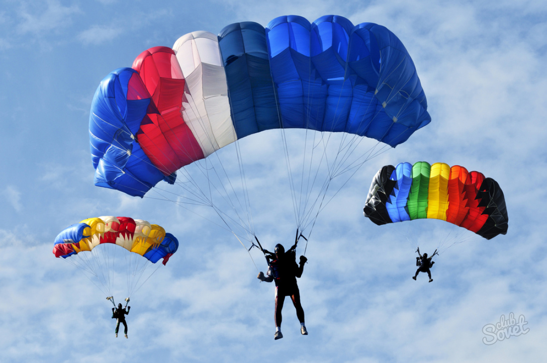
Как найти силу сопротивления
При движении любого предмета по поверхности или в воздухе возникают силы, препятствующие этому. Их называют силами сопротивления или трения. В этой статье мы расскажем, как найти силу сопротивления, и рассмотрим факторы, влияющие на нее.
1
Для определения силы сопротивления необходимо воспользоваться третьим законом Ньютона. Эта величина численно равна силе, которую нужно приложить, чтобы заставить равномерно двигаться предмет по ровной горизонтальной поверхности. Это можно сделать при помощи динамометра.

2
Сила сопротивления вычисляется по формуле F=μ*m*g. Согласно этой формуле, искомая величина прямо пропорциональна массе тела. Стоит учесть, что для правильного подсчета необходимо выбрать μ – коэффициент, зависящий от материала, из которого изготовлена опора. Принимают во внимание и материал предмета. Этот коэффициент выбирается по таблице. Для расчета используется постоянная g, которая равна 9,8 м/с2.
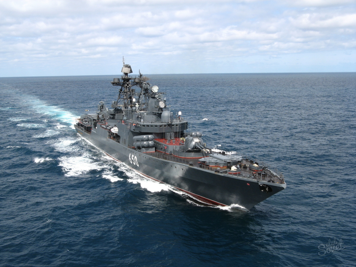
3
Как рассчитать сопротивление, если тело движется не прямолинейно, а по наклонной плоскости? Для этого в первоначальную формулу нужно ввести cos угла. Именно от угла наклона зависит трение и сопротивление поверхности тел к движению. Формула для определения трения по наклонной плоскости будет иметь такой вид: F=μ*m*g*cos(α).

4
Если тело движется на высоте, то на него действует сила трения воздуха, которая зависит от скорости движения предмета. Искомую величину можно рассчитать по формуле F=v*α. Где v – скорость движения предмета, а α – коэффициент сопротивления среды. Эта формула подходит исключительно для тел, которые передвигаются с небольшой скоростью. Для определения силы сопротивления реактивных самолетов и других высокоскоростных агрегатов применяют другую – F=v2*β. Для расчета силы трения высокоскоростных тел используют квадрат скорости и коэффициент β, который рассчитывается для каждого предмета отдельно. При движении предмета в газе или жидкости при расчете силы трения необходимо учитывать плотность среды, а также массу и объем тела.
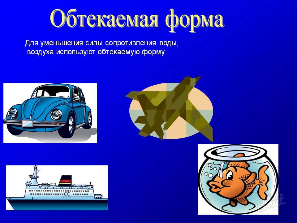
5
Сопротивление движению существенно снижает скорость поездов и автомобилей. Причем на движущие предметы действует два вида сил – постоянные и временные. Общая сила трения представлена суммой двух величин. Для снижения сопротивления и повышения скорости машины конструкторы и инженеры изобретают разнообразные материалы со скользящей поверхностью, от которой воздух отталкивается. Именно поэтому передняя часть скоростных поездов имеет обтекаемую форму. Рыбы очень быстро движутся в воде благодаря обтекаемому телу, покрытому слизью, которая снижает трение.

6
Не всегда сила сопротивления отрицательно сказывается на движении машин. Чтобы вытащить автомобиль из грязи, необходимо под колеса насыпать песок или щебень. Благодаря увеличению трения авто отлично справляется с болотистой почвой и грязью.

Сопротивление движения в воздухе используется во время прыжков с парашютом. В результате возникающего трения между куполом и воздухом скорость движения парашютиста снижается, что позволяет без ущерба для жизни заниматься парашютным спортом.