Как пишется степень в математике - Граматика и образование на Pisanino.ru

В рамках этого материала мы разберем, что такое степень числа. Помимо основных определений мы сформулируем, что такое степени с натуральными, целыми, рациональными и иррациональными показателями. Как всегда, все понятия будут проиллюстрированы примерами задач.

Степени с натуральными показателями: понятие квадрата и куба числа

Сначала сформулируем базовое определение степени с натуральным показателем. Для этого нам понадобится вспомнить основные правила умножения. Заранее уточним, что в качестве основания будем пока брать действительное число (обозначим его буквой a), а в качестве показателя – натуральное (обозначим буквой n).

Определение 1

Степень числа a с натуральным показателем n – это произведение n-ного числа множителей, каждый из которых равен числу а. Записывается степень так: an, а в виде формулы ее состав можно представить следующим образом:

Например, если показатель степени равен 1, а основание – a, то первая степень числа a записывается как a1. Учитывая, что a – это значение множителя, а 1 – число множителей, мы можем сделать вывод, что a1=a.

В целом можно сказать, что степень – это удобная форма записи большого количества равных множителей. Так, запись вида 8·8·8·8 можно сократить до 84. Примерно так же произведение помогает нам избежать записи большого числа слагаемых (8+8+8+8=8·4); мы это уже разбирали в статье, посвященной умножению натуральных чисел.

Как же верно прочесть запись степени? Общепринятый вариант – «a в степени n». Или можно сказать «n-ная степень a» либо «a n-ной степени». Если, скажем, в примере встретилась запись 812, мы можем прочесть «8 в 12-й степени», «8 в степени 12» или «12-я степень 8-ми».

Вторая и третья степени числа имеют свои устоявшиеся названия: квадрат и куб. Если мы видим вторую степень, например, числа 7(72), то мы можем сказать «7 в квадрате» или «квадрат числа 7». Аналогично третья степень читается так: 53 – это «куб числа 5» или «5 в кубе». Впрочем, употреблять стандартную формулировку «во второй/третьей степени» тоже можно, это не будет ошибкой.

Пример 1

Разберем пример степени с натуральным показателем: для 57 пятерка будет основанием, а семерка – показателем.

В основании не обязательно должно стоять целое число: для степени (4,32)9 основанием будет дробь 4,32, а показателем – девятка. Обратите внимание на скобки: такая запись делается для всех степеней, основания которых отличаются от натуральных чисел.

Например: 123, (-3)12, -2352, 2,4355, 73.

Для чего нужны скобки? Они помогают избежать ошибок в расчетах. Скажем, у нас есть две записи: (−2)3 и −23. Первая из них означает отрицательное число минус два, возведенное в степень с натуральным показателем три; вторая – число, соответствующее противоположному значению степени 23.

Иногда в книгах можно встретить немного другое написание степени числа – a^n (где а – основание, а n — показатель). То есть 4^9 – это то же самое, что и 49. В случае, если n представляет собой многозначное число, оно берется в скобки. Например, 15^ (21), (−3,1) ^ (156). Но мы будем использовать обозначение anкак более употребительное.

О том, как вычислить значение степени с натуральным показателем, легко догадаться из ее определения: нужно просто перемножить a n-ное число раз. Подробнее об этом мы писали в другой статье.

Понятие степени является обратным другому математическому понятию – корню числа. Если мы знаем значение степени и показатель, мы можем вычислить ее основание. Степень обладает некоторыми специфическими свойствами, полезными для решения задач, которые мы разобрали в рамках отдельного материала.

Что такое степени с целым показателем

В показателях степени могут стоять не только натуральные числа, но и вообще любые целые значения, в том числе отрицательные и нули, ведь они тоже принадлежат к множеству целых чисел.

Определение 2

Степень числа с целым положительным показателем можно отобразить в виде формулы: .

При этом n – любое целое положительное число.

Разберемся с понятием нулевой степени. Для этого мы используем подход, учитывающий свойство частного для степеней с равными основаниями. Оно формулируется так:

Определение 3

Равенство am:an=am−n будет верно при условиях: m и n – натуральные числа, m <n, a≠0.

Последнее условие важно, поскольку позволяет избежать деления на ноль. Если значения m и n равны, то мы получим следующий результат: an:an=an−n=a0

Но при этом an:an=1 — частное равных чисел an и a. Выходит, что нулевая степень любого отличного от нуля числа равна единице.

Однако такое доказательство не подходит для нуля в нулевой степени. Для этого нам нужно другое свойство степеней – свойство произведений степеней с равными основаниями. Оно выглядит так: am·an=am+n .

Если n у нас равен 0, то am·a0=am (такое равенство также доказывает нам, что a0=1). Но если а также равно нулю, наше равенство приобретает вид 0m·00=0m, Оно будет верным при любом натуральном значении n, и неважно при этом, чему именно равно значение степени 00, то есть оно может быть равно любому числу, и на верность равенства это не повлияет. Следовательно, запись вида 00 своего особенного смысла не имеет, и мы не будем ему его приписывать.

При желании легко проверить, что a0=1 сходится со свойством степени (am)n=am·n при условии, что основание степени не равно нулю. Таким образом, степень любого отличного от нуля числа с нулевым показателем равна единице.

Пример 2

Разберем пример с конкретными числами: Так, 50 — единица, (33,3)0=1, -4590=1, а значение 00не определено.

После нулевой степени нам осталось разобраться, что из себя представляет степень отрицательная. Для этого нам понадобится то же свойство произведения степеней с равными основаниями, которое мы уже использовали выше: am·an=am+n.

Введем условие: m=−n, тогда a не должно быть равно нулю. Из этого следует, что a−n·an=a−n+n=a0=1. Выходит, что an и a−n у нас являются взаимно обратными числами.

В итоге a в целой отрицательной степени есть не что иное, как дробь 1an.

Такая формулировка подтверждает, что для степени с целым отрицательным показателем действительны все те же свойства, которыми обладает степень с натуральным показателем (при условии, что основание не равно нулю).

Пример 3

Степень a с целым отрицательным показателем n можно представить в виде дроби 1an. Таким образом, a-n=1an при условии a≠0 и n – любое натуральное число.

Проиллюстрируем нашу мысль конкретными примерами:

Пример 4

3-2=132, (-4.2)-5=1(-4.2)5, 1137-1=111371

В последней части параграфа попробуем изобразить все сказанное наглядно в одной формуле:

Определение 4

Степень числа a с натуральным показателем z – это: az=az, eсли z-целое положительное число1, z=0 и a≠0, (при z=0 и a=0 получается 00, значения выражения 00 не определяется) 1az, если z — целое отрицательное число и a≠0 (если z — целое отрицательное число и a=0 получается 0z, его значение не определяется)

Что такое степени с рациональным показателем

Мы разобрали случаи, когда в показателе степени стоит целое число. Однако возвести число в степень можно и тогда, когда в ее показателе стоит дробное число. Это называется степенью с рациональным показателем. В этом пункте мы докажем, что она обладает теми же свойствами, что и другие степени.

Что такое рациональные числа? В их множество входят как целые, так и дробные числа, при этом дробные числа можно представить в виде обыкновенных дробей (как положительных, так и отрицательных). Сформулируем определение степени числа a с дробным показателем m/n, где n – натуральное число, а m – целое.

У нас есть некоторая степень с дробным показателем amn. Для того, чтобы свойство степени в степени выполнялось, равенство amnn=amn·n=am должно быть верным.

Учитывая определение корня n-ной степени и что amnn=am, мы можем принять условие amn=amn, если amn имеет смысл при данных значениях m, n и a.

Приведенные выше свойства степени с целым показателем будут верными при условии amn=amn.

Основной вывод из наших рассуждений таков: степень некоторого числа a с дробным показателем m/n – это корень n-ой степени из числа a в степени m. Это справедливо в том случае, если при данных значениях m, n и a выражение amn сохраняет смысл.

Далее нам необходимо определить, какие именно ограничения на значения переменных накладывает такое условие. Есть два подхода к решению этой проблемы.

1. Мы можем ограничить значение основания степени: возьмем a, которое при положительных значениях m будет больше или равно 0, а для отрицательных – строго меньше (поскольку при m≤0 мы получаем 0m, а такая степень не определена). В таком случае определение степени с дробным показателем будет выглядеть следующим образом:

Степень с дробным показателем m/n для некоторого положительного числа a есть корень n-ной степени из a, возведенного в степень m. В виде формулы это можно изобразить так:

amn=amn

Для степени с нулевым основанием это положение также подходит, но только в том случае, если ее показатель – положительное число.

Степень с нулевым основанием и дробным положительным показателем m/n можно выразить как

0mn=0mn=0 при условии целого положительного m и натурального n.

При отрицательном отношении mn<0 степень не определяется, т.е. такая запись смысла не имеет.

Отметим один момент. Поскольку мы ввели условие, что a больше или равно нулю, то у нас оказались отброшены некоторые случаи.

Выражение amn иногда все же имеет смысл при некоторых отрицательных значениях a и некоторых m. Так, верны записи (-5)23, (-1,2)57, -12-84, в которых основание отрицательно.

2. Второй подход – это рассмотреть отдельно корень amn с четными и нечетными показателями. Тогда нам потребуется ввести еще одно условие: степень a, в показателе которой стоит сократимая обыкновенная дробь, считается степенью a, в показателе которой стоит соответствующая ей несократимая дробь. Позже мы объясним, для чего нам это условие и почему оно так важно. Таким образом, если у нас есть запись am·kn·k, то мы можем свести ее к amn и упростить расчеты.

Если n – нечетное число, а значение m – положительно, a – любое неотрицательное число, то amn имеет смысл. Условие неотрицательного a нужно, поскольку корень четной степени из отрицательного числа не извлекают. Если же значение m положительно, то a может быть и отрицательным, и нулевым, т.к. корень нечетной степени можно извлечь из любого действительного числа.

Объединим все данные выше определения в одной записи:

Здесь m/n означает несократимую дробь, m – любое целое число, а n – любое натуральное число.

Определение 5

Для любой обыкновенной сократимой дроби m·kn·k степень можно заменить на amn.

Степень числа a с несократимым дробным показателем m/n – можно выразить в виде amn в следующих случаях: — для любых действительных a, целых положительных значений m и нечетных натуральных значений n. Пример: 253=253, (-5,1)27=(-5,1)-27, 0519=0519.

— для любых отличных от нуля действительных a, целых отрицательных значений m и нечетных значений n, например, 2-53=2-53, (-5,1)-27=(-5,1)-27

— для любых неотрицательных a, целых положительных значений m и четных n, например, 214=214, (5,1)32=(5,1)3, 0718=0718.

— для любых положительных a, целых отрицательных m и четных n, например, 2-14=2-14, (5,1)-32=(5,1)-3, .

В случае других значений степень с дробным показателем не определяется. Примеры таких степеней: -2116, -21232, 0-25.

Теперь объясним важность условия, о котором говорили выше: зачем заменять дробь с сократимым показателем на дробь с несократимым. Если бы мы этого не сделали бы, то получились бы такие ситуации, скажем, 6/10=3/5. Тогда должно быть верным (-1)610=-135, но -1610=(-1)610=110=11010=1, а (-1)35=(-1)35=-15=-155=-1.

Определение степени с дробным показателем, которое мы привели первым, удобнее применять на практике, чем второе, поэтому мы будем далее пользоваться именно им.

Определение 6

Таким образом, степень положительного числа a с дробным показателем m/n определяется как 0mn=0mn=0. В случае отрицательных a запись amn не имеет смысла. Степень нуля для положительных дробных показателей m/n определяется как 0mn=0mn=0, для отрицательных дробных показателей мы степень нуля не определяем.

В выводах отметим, что можно записать любой дробный показатель как в виде смешанного числа, так и в виде десятичной дроби: 51,7, 325-237.

При вычислении же лучше заменять показатель степени обыкновенной дробью и далее пользоваться определением степени с дробным показателем. Для примеров выше у нас получится:

51,7=51710=5710325-237=325-177=325-177

Что такое степени с иррациональным и действительным показателем

Что такое действительные числа? В их множество входят как рациональные, так и иррациональные числа. Поэтому для того, чтобы понять, что такое степень с действительным показателем, нам надо определить степени с рациональными и иррациональными показателями. Про рациональные мы уже упоминали выше. Разберемся с иррациональными показателями пошагово.

Пример 5

Допустим, что у нас есть иррациональное число a и последовательность его десятичных приближений a0, a1, a2, …. Например, возьмем значение a=1,67175331…,тогда

a0=1,6, a1=1,67, a2=1,671, …,a0=1,67, a1=1,6717, a2=1,671753, …

и так далее (при этом сами приближения являются рациональными числами).

Последовательности приближений мы можем поставить в соответствие последовательность степеней aa0, aa1, aa2, …. Если вспомнить, что мы рассказывали ранее о возведении чисел в рациональную степень, то мы можем сами подсчитать значения этих степеней.

Возьмем для примера a=3, тогда aa0=31,67, aa1=31,6717, aa2=31,671753, … и т.д.

Последовательность степеней можно свести к числу, которое и будет значением степени c основанием a и иррациональным показателем a. В итоге : степень с иррациональным показателем вида 31,67175331.. можно свести к числу 6,27.

Определение 7

Степень положительного числа a с иррациональным показателем a записывается как aa. Его значение – это предел последовательности aa0, aa1, aa2, …, где a0, a1, a2, … являются последовательными десятичными приближениями иррационального числа a. Степень с нулевым основанием можно определить и для положительных иррациональных показателей, при этом 0a=0 Так, 06=0,02133=0. А для отрицательных этого сделать нельзя, поскольку, например, значение 0-5, 0-2π не определено. Единица, возведенная в любую иррациональную степень, остается единицей, например, и 12, 15в2 и 1-5 будут равны 1.

Источник

bⁿ
notation
base b and exponent n

Graphs of y = b^x for various bases b: base 10, base e, base 2, base 1/2. Each curve passes through the point (0, 1) because any nonzero number raised to the power of 0 is 1. At x = 1, the value of y equals the base because any number raised to the power of 1 is the number itself.

Exponentiation is a mathematical operation, written as bⁿ, involving two numbers, the base b and the exponent or power n, and pronounced as «b (raised) to the (power of) n«.^[1] When n is a positive integer, exponentiation corresponds to repeated multiplication of the base: that is, bⁿ is the product of multiplying n bases:^[1]

${displaystyle b^{n}=underbrace {btimes btimes dots times btimes b} _{n{text{ times}}}.}$

The exponent is usually shown as a superscript to the right of the base. In that case, bⁿ is called «b raised to the nth power», «b (raised) to the power of n«, «the nth power of b«, «b to the nth power»,^[2] or most briefly as «b to the nth».

Starting from the basic fact stated above that, for any positive integer , $b^{n}$ is occurrences of all multiplied by each other, several other properties of exponentiation directly follow. In particular:^{[nb 1]}

${displaystyle {begin{aligned}b^{n+m}&=underbrace {btimes dots times b} _{n+m{text{ times}}}\[1ex]&=underbrace {btimes dots times b} _{n{text{ times}}}times underbrace {btimes dots times b} _{m{text{ times}}}\[1ex]&=b^{n}times b^{m}end{aligned}}}$

In other words, when multiplying a base raised to one exponent by the same base raised to another exponent, the exponents add. From this basic rule that exponents add, we can derive that $b^{0}$ must be equal to 1, as follows. For any , ${displaystyle b^{0}cdot b^{n}=b^{0+n}=b^{n}}$ . Dividing both sides by $b^{n}$ gives ${displaystyle b^{0}=b^{n}/b^{n}=1}$ .

The fact that $b^{1}=b$ can similarly be derived from the same rule. For example, ${displaystyle (b^{1})^{3}=b^{1}cdot b^{1}cdot b^{1}=b^{1+1+1}=b^{3}}$ . Taking the cube root of both sides gives $b^{1}=b$ .

The rule that multiplying makes exponents add can also be used to derive the properties of negative integer exponents. Consider the question of what $b^{-1}$ should mean. In order to respect the «exponents add» rule, it must be the case that ${displaystyle b^{-1}cdot b^{1}=b^{-1+1}=b^{0}=1}$ . Dividing both sides by ${displaystyle b^{1}}$ gives ${displaystyle b^{-1}=1/b^{1}}$ , which can be more simply written as ${displaystyle b^{-1}=1/b}$ , using the result from above that $b^{1}=b$ . By a similar argument, ${displaystyle b^{-n}=1/b^{n}}$ .

The properties of fractional exponents also follow from the same rule. For example, suppose we consider sqrt{b} and ask if there is some suitable exponent, which we may call , such that ${displaystyle b^{r}={sqrt {b}}}$ . From the definition of the square root, we have that . Therefore, the exponent must be such that ${displaystyle b^{r}cdot b^{r}=b}$ . Using the fact that multiplying makes exponents add gives ${displaystyle b^{r+r}=b}$ . The on the right-hand side can also be written as ${displaystyle b^{1}}$ , giving ${displaystyle b^{r+r}=b^{1}}$ . Equating the exponents on both sides, we have . Therefore, $r={frac {1}{2}}$ , so ${displaystyle {sqrt {b}}=b^{1/2}}$ .

The definition of exponentiation can be extended to allow any real or complex exponent. Exponentiation by integer exponents can also be defined for a wide variety of algebraic structures, including matrices.

Exponentiation is used extensively in many fields, including economics, biology, chemistry, physics, and computer science, with applications such as compound interest, population growth, chemical reaction kinetics, wave behavior, and public-key cryptography.

History of the notation[edit]

The term power (Latin: potentia, potestas, dignitas) is a mistranslation^[3]^[4] of the ancient Greek δύναμις (dúnamis, here: «amplification»^[3]) used by the Greek mathematician Euclid for the square of a line,^[5] following Hippocrates of Chios.^[6] In The Sand Reckoner, Archimedes discovered and proved the law of exponents, 10^a · 10^b = 10^a+b, necessary to manipulate powers of 10.^{[citation needed]} In the 9th century, the Persian mathematician Muhammad ibn Mūsā al-Khwārizmī used the terms مَال (māl, «possessions», «property») for a square—the Muslims, «like most mathematicians of those and earlier times, thought of a squared number as a depiction of an area, especially of land, hence property»^[7]—and كَعْبَة (kaʿbah, «cube») for a cube, which later Islamic mathematicians represented in mathematical notation as the letters mīm (m) and kāf (k), respectively, by the 15th century, as seen in the work of Abū al-Hasan ibn Alī al-Qalasādī.^[8]

In the late 16th century, Jost Bürgi used Roman numerals for exponents.^[9]

Nicolas Chuquet used a form of exponential notation in the 15th century, which was later used by Henricus Grammateus and Michael Stifel in the 16th century. The word exponent was coined in 1544 by Michael Stifel.^[10]^[11] Samuel Jeake introduced the term indices in 1696.^[5] In the 16th century, Robert Recorde used the terms square, cube, zenzizenzic (fourth power), sursolid (fifth), zenzicube (sixth), second sursolid (seventh), and zenzizenzizenzic (eighth).^[7] Biquadrate has been used to refer to the fourth power as well.

Early in the 17th century, the first form of our modern exponential notation was introduced by René Descartes in his text titled La Géométrie; there, the notation is introduced in Book I.^[12]

Some mathematicians (such as René Descartes) used exponents only for powers greater than two, preferring to represent squares as repeated multiplication. Thus they would write polynomials, for example, as ax + bxx + cx³ + d.

Another historical synonym,^{[clarification needed]} involution, is now rare^[13] and should not be confused with its more common meaning.

In 1748, Leonhard Euler introduced variable exponents, and, implicitly, non-integer exponents by writing:

«consider exponentials or powers in which the exponent itself is a variable. It is clear that quantities of this kind are not algebraic functions, since in those the exponents must be constant.»^[14]

Terminology[edit]

The expression b² = b · b is called «the square of b» or «b squared», because the area of a square with side-length b is b².

Similarly, the expression b³ = b · b · b is called «the cube of b» or «b cubed», because the volume of a cube with side-length b is b³.

When it is a positive integer, the exponent indicates how many copies of the base are multiplied together. For example, 3⁵ = 3 · 3 · 3 · 3 · 3 = 243. The base 3 appears 5 times in the multiplication, because the exponent is 5. Here, 243 is the 5th power of 3, or 3 raised to the 5th power.

The word «raised» is usually omitted, and sometimes «power» as well, so 3⁵ can be simply read «3 to the 5th», or «3 to the 5». Therefore, the exponentiation bⁿ can be expressed as «b to the power of n«, «b to the nth power», «b to the nth», or most briefly as «b to the n«.

A formula with nested exponentiation, such as 3^5⁷ (which means 3^(5⁷) and not (3⁵)⁷), is called a tower of powers, or simply a tower.^[15] For example writing ${displaystyle b^{c^{d}}}$ is equivalent to writing ${displaystyle b^{left(c^{d}right)}}$ . This can be generalized to where writing ${displaystyle b^{c^{d^{f}}}}$ means ${displaystyle b^{left(c^{left(d^{f}right)}right)}}$ . For example, can be computed as ${displaystyle 100^{frac {1}{2}}}$ , which can be computed as ${displaystyle 100^{2^{-1}}}$ , which is equal to ${displaystyle 100^{left(2^{-1}right)}}$ , which is equal to 10..

Integer exponents[edit]

The exponentiation operation with integer exponents may be defined directly from elementary arithmetic operations.

Positive exponents[edit]

The definition of the exponentiation as an iterated multiplication can be formalized by using induction,^[16] and this definition can be used as soon one has an associative multiplication:

The base case is

$b^{1}=b$

and the recurrence is

${displaystyle b^{n+1}=b^{n}cdot b.}$

The associativity of multiplication implies that for any positive integers m and n,

${displaystyle b^{m+n}=b^{m}cdot b^{n},}$

and

${displaystyle (b^{m})^{n}=b^{mn}.}$

Zero exponent[edit]

By definition, any nonzero number raised to the 0 power is 1:^[17]^[1]

${displaystyle b^{0}=1.}$

This definition is the only possible that allows extending the formula

${displaystyle b^{m+n}=b^{m}cdot b^{n}}$

to zero exponents. It may be used in every algebraic structure with a multiplication that has an identity.

Intuitionally, $b^{0}$ may be interpreted as the empty product of copies of b. So, the equality $b^{0}=1$ is a special case of the general convention for the empty product.

The case of 0⁰ is more complicated. In contexts where only integer powers are considered, the value 1 is generally assigned to ${displaystyle 0^{0},}$ but, otherwise, the choice of whether to assign it a value and what value to assign may depend on context. For more details, see Zero to the power of zero.

Negative exponents[edit]

Exponentiation with negative exponents is defined by the following identity, which holds for any integer n and nonzero b:

${displaystyle b^{-n}={frac {1}{b^{n}}}}$

.^[1]

Raising 0 to a negative exponent is undefined but, in some circumstances, it may be interpreted as infinity ( infty ).^{[citation needed]}

This definition of exponentiation with negative exponents is the only one that allows extending the identity ${displaystyle b^{m+n}=b^{m}cdot b^{n}}$ to negative exponents (consider the case ).

The same definition applies to invertible elements in a multiplicative monoid, that is, an algebraic structure, with an associative multiplication and a multiplicative identity denoted 1 (for example, the square matrices of a given dimension). In particular, in such a structure, the inverse of an invertible element x is standardly denoted $x^{{-1}}.$

Identities and properties[edit]

The following identities, often called exponent rules, hold for all integer exponents, provided that the base is non-zero:^[1]

${displaystyle {begin{aligned}b^{m+n}&=b^{m}cdot b^{n}\left(b^{m}right)^{n}&=b^{mcdot n}\(bcdot c)^{n}&=b^{n}cdot c^{n}end{aligned}}}$

Unlike addition and multiplication, exponentiation is not commutative. For example, 2³ = 8 ≠ 3² = 9. Also unlike addition and multiplication, exponentiation is not associative. For example, (2³)² = 8² = 64, whereas 2^(3²) = 2⁹ = 512. Without parentheses, the conventional order of operations for serial exponentiation in superscript notation is top-down (or right-associative), not bottom-up^[18]^[19]^[20]^[21] (or left-associative). That is,

${displaystyle b^{p^{q}}=b^{left(p^{q}right)},}$

which, in general, is different from

${displaystyle left(b^{p}right)^{q}=b^{pq}.}$

Powers of a sum[edit]

The powers of a sum can normally be computed from the powers of the summands by the binomial formula

${displaystyle (a+b)^{n}=sum _{i=0}^{n}{binom {n}{i}}a^{i}b^{n-i}=sum _{i=0}^{n}{frac {n!}{i!(n-i)!}}a^{i}b^{n-i}.}$

However, this formula is true only if the summands commute (i.e. that ab = ba), which is implied if they belong to a structure that is commutative. Otherwise, if a and b are, say, square matrices of the same size, this formula cannot be used. It follows that in computer algebra, many algorithms involving integer exponents must be changed when the exponentiation bases do not commute. Some general purpose computer algebra systems use a different notation (sometimes ^^ instead of ^) for exponentiation with non-commuting bases, which is then called non-commutative exponentiation.

Combinatorial interpretation[edit]

n^m	The n^m possible m-tuples of elements from the set {1, …, n}
0⁵ = 0	none
1⁴ = 1	(1, 1, 1, 1)
2³ = 8	(1, 1, 1), (1, 1, 2), (1, 2, 1), (1, 2, 2), (2, 1, 1), (2, 1, 2), (2, 2, 1), (2, 2, 2)
3² = 9	(1, 1), (1, 2), (1, 3), (2, 1), (2, 2), (2, 3), (3, 1), (3, 2), (3, 3)
4¹ = 4	(1), (2), (3), (4)
5⁰ = 1	()

Particular bases[edit]

Powers of ten[edit]

In the base ten (decimal) number system, integer powers of 10 are written as the digit 1 followed or preceded by a number of zeroes determined by the sign and magnitude of the exponent. For example, 10³ = 1000 and 10⁻⁴ = 0.0001.

Exponentiation with base 10 is used in scientific notation to denote large or small numbers. For instance, 299792458 m/s (the speed of light in vacuum, in metres per second) can be written as 2.99792458×10⁸ m/s and then approximated as 2.998×10⁸ m/s.

SI prefixes based on powers of 10 are also used to describe small or large quantities. For example, the prefix kilo means 10³ = 1000, so a kilometre is 1000 m.

Powers of two[edit]

The first negative powers of 2 are commonly used, and have special names, e.g.: half and quarter.

Powers of 2 appear in set theory, since a set with n members has a power set, the set of all of its subsets, which has 2ⁿ members.

Integer powers of 2 are important in computer science. The positive integer powers 2ⁿ give the number of possible values for an n-bit integer binary number; for example, a byte may take 2⁸ = 256 different values. The binary number system expresses any number as a sum of powers of 2, and denotes it as a sequence of 0 and 1, separated by a binary point, where 1 indicates a power of 2 that appears in the sum; the exponent is determined by the place of this 1: the nonnegative exponents are the rank of the 1 on the left of the point (starting from 0), and the negative exponents are determined by the rank on the right of the point.

Powers of one[edit]

Every power of one equals: 1ⁿ = 1. This is true even if n is negative.

The first power of a number is the number itself: ${displaystyle n^{1}=n.}$

Powers of zero[edit]

If the exponent n is positive (n > 0), the nth power of zero is zero: 0ⁿ = 0.

If the exponent n is negative (n < 0), the nth power of zero 0ⁿ is undefined, because it must equal ${displaystyle 1/0^{-n}}$ with −n > 0, and this would be 1/0 according to above.

The expression 0⁰ is either defined as 1, or it is left undefined.

Powers of negative one[edit]

If n is an even integer, then (−1)ⁿ = 1. This is because a negative number multiplied by another negative number cancels out, and gives a positive number.

If n is an odd integer, then (−1)ⁿ = −1. This is because there will be a remaining (-1) after removing all (-1) pairs.

Because of this, powers of −1 are useful for expressing alternating sequences. For a similar discussion of powers of the complex number i, see § nth roots of a complex number.

Large exponents[edit]

The limit of a sequence of powers of a number greater than one diverges; in other words, the sequence grows without bound:

bⁿ → ∞ as n → ∞ when b > 1

This can be read as «b to the power of n tends to +∞ as n tends to infinity when b is greater than one».

Powers of a number with absolute value less than one tend to zero:

bⁿ → 0 as n → ∞ when |b| < 1

Any power of one is always one:

bⁿ = 1 for all n if b = 1

Powers of –1 alternate between 1 and –1 as n alternates between even and odd, and thus do not tend to any limit as n grows.

If b < –1, bⁿ alternates between larger and larger positive and negative numbers as n alternates between even and odd, and thus does not tend to any limit as n grows.

If the exponentiated number varies while tending to 1 as the exponent tends to infinity, then the limit is not necessarily one of those above. A particularly important case is

(1 + 1/n)ⁿ → e as n → ∞

See § The exponential function below.

Other limits, in particular those of expressions that take on an indeterminate form, are described in § Limits of powers below.

Power functions[edit]

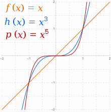
Power functions for

Real functions of the form ${displaystyle f(x)=cx^{n}}$ , where cneq 0 , are sometimes called power functions.^[22] When is an integer and ngeq 1 , two primary families exist: for even, and for odd. In general for c>0 , when is even ${displaystyle f(x)=cx^{n}}$ will tend towards positive infinity with increasing , and also towards positive infinity with decreasing . All graphs from the family of even power functions have the general shape of ${displaystyle y=cx^{2}}$ , flattening more in the middle as increases.^[23] Functions with this kind of symmetry () are called even functions.

When is odd, f(x) ‘s asymptotic behavior reverses from positive to negative . For c>0 , ${displaystyle f(x)=cx^{n}}$ will also tend towards positive infinity with increasing , but towards negative infinity with decreasing . All graphs from the family of odd power functions have the general shape of ${displaystyle y=cx^{3}}$ , flattening more in the middle as increases and losing all flatness there in the straight line for n=1 . Functions with this kind of symmetry () are called odd functions.

For c < 0 , the opposite asymptotic behavior is true in each case.^[23]

Table of powers of decimal digits[edit]

n	n²	n³	n⁴	n⁵	n⁶	n⁷	n⁸	n⁹	n¹⁰
1	1	1	1	1	1	1	1	1	1
2	4	8	16	32	64	128	256	512	1024
3	9	27	81	243	729	2187	6561	19683	59049
4	16	64	256	1024	4096	16384	65536	262144	1048576
5	25	125	625	3125	15625	78125	390625	1953125	9765625
6	36	216	1296	7776	46656	279936	1679616	10077696	60466176
7	49	343	2401	16807	117649	823543	5764801	40353607	282475249
8	64	512	4096	32768	262144	2097152	16777216	134217728	1073741824
9	81	729	6561	59049	531441	4782969	43046721	387420489	3486784401
10	100	1000	10000	100000	1000000	10000000	100000000	1000000000	10000000000

Rational exponents[edit]

From top to bottom: x^1/8, x^1/4, x^1/2, x¹, x², x⁴, x⁸.

If x is a nonnegative real number, and n is a positive integer, $x^{1/n}$ or denotes the unique positive real nth root of x, that is, the unique positive real number y such that ${displaystyle y^{n}=x.}$

If x is a positive real number, and ${frac pq}$ is a rational number, with p and q ≠ 0 integers, then ${textstyle x^{p/q}}$ is defined as

${displaystyle x^{frac {p}{q}}=left(x^{p}right)^{frac {1}{q}}=(x^{frac {1}{q}})^{p}.}$

The equality on the right may be derived by setting ${displaystyle y=x^{frac {1}{q}},}$ and writing ${displaystyle (x^{frac {1}{q}})^{p}=y^{p}=left((y^{p})^{q}right)^{frac {1}{q}}=left((y^{q})^{p}right)^{frac {1}{q}}=(x^{p})^{frac {1}{q}}.}$

If r is a positive rational number, ${displaystyle 0^{r}=0,}$ by definition.

All these definitions are required for extending the identity ${displaystyle (x^{r})^{s}=x^{rs}}$ to rational exponents.

On the other hand, there are problems with the extension of these definitions to bases that are not positive real numbers. For example, a negative real number has a real nth root, which is negative, if n is odd, and no real root if n is even. In the latter case, whichever complex nth root one chooses for ${displaystyle x^{frac {1}{n}},}$ the identity ${displaystyle (x^{a})^{b}=x^{ab}}$ cannot be satisfied. For example,

${displaystyle left((-1)^{2}right)^{frac {1}{2}}=1^{frac {1}{2}}=1neq (-1)^{2cdot {frac {1}{2}}}=(-1)^{1}=-1.}$

See § Real exponents and § Non-integer powers of complex numbers for details on the way these problems may be handled.

Real exponents[edit]

For positive real numbers, exponentiation to real powers can be defined in two equivalent ways, either by extending the rational powers to reals by continuity (§ Limits of rational exponents, below), or in terms of the logarithm of the base and the exponential function (§ Powers via logarithms, below). The result is always a positive real number, and the identities and properties shown above for integer exponents remain true with these definitions for real exponents. The second definition is more commonly used, since it generalizes straightforwardly to complex exponents.

On the other hand, exponentiation to a real power of a negative real number is much more difficult to define consistently, as it may be non-real and have several values (see § Real exponents with negative bases). One may choose one of these values, called the principal value, but there is no choice of the principal value for which the identity

${displaystyle left(b^{r}right)^{s}=b^{rs}}$

is true; see § Failure of power and logarithm identities. Therefore, exponentiation with a basis that is not a positive real number is generally viewed as a multivalued function.

Limits of rational exponents[edit]

The limit of e^1/n is e⁰ = 1 when n tends to the infinity.

Since any irrational number can be expressed as the limit of a sequence of rational numbers, exponentiation of a positive real number b with an arbitrary real exponent x can be defined by continuity with the rule^[24]

${displaystyle b^{x}=lim _{r(in mathbb {Q} )to x}b^{r}quad (bin mathbb {R} ^{+},,xin mathbb {R} ),}$

where the limit is taken over rational values of r only. This limit exists for every positive b and every real x.

For example, if x = π, the non-terminating decimal representation π = 3.14159… and the monotonicity of the rational powers can be used to obtain intervals bounded by rational powers that are as small as desired, and must contain ${displaystyle b^{pi }:}$

${displaystyle left[b^{3},b^{4}right],left[b^{3.1},b^{3.2}right],left[b^{3.14},b^{3.15}right],left[b^{3.141},b^{3.142}right],left[b^{3.1415},b^{3.1416}right],left[b^{3.14159},b^{3.14160}right],ldots }$

So, the upper bounds and the lower bounds of the intervals form two sequences that have the same limit, denoted ${displaystyle b^{pi }.}$

This defines b^x for every positive b and real x as a continuous function of b and x. See also Well-defined expression.^[25]

The exponential function[edit]

The exponential function is often defined as ${displaystyle xmapsto e^{x},}$ where is Euler’s number. For avoiding circular reasoning, this definition cannot be used here. So, a definition of the exponential function, denoted and of Euler’s number are given, which rely only on exponentiation with positive integer exponents. Then a proof is sketched that, if one uses the definition of exponentiation given in preceding sections, one has

${displaystyle exp(x)=e^{x}.}$

There are many equivalent ways to define the exponential function, one of them being

${displaystyle exp(x)=lim _{nrightarrow infty }left(1+{frac {x}{n}}right)^{n}.}$

One has and the exponential identity holds as well, since

${displaystyle exp(x)exp(y)=lim _{nrightarrow infty }left(1+{frac {x}{n}}right)^{n}left(1+{frac {y}{n}}right)^{n}=lim _{nrightarrow infty }left(1+{frac {x+y}{n}}+{frac {xy}{n^{2}}}right)^{n},}$

and the second-order term ${displaystyle {frac {xy}{n^{2}}}}$ does not affect the limit, yielding .

Euler’s number can be defined as . It follows from the preceding equations that ${displaystyle exp(x)=e^{x}}$ when x is an integer (this results from the repeated-multiplication definition of the exponentiation). If x is real, ${displaystyle exp(x)=e^{x}}$ results from the definitions given in preceding sections, by using the exponential identity if x is rational, and the continuity of the exponential function otherwise.

The limit that defines the exponential function converges for every complex value of x, and therefore it can be used to extend the definition of , and thus ${displaystyle e^{z},}$ from the real numbers to any complex argument z. This extended exponential function still satisfies the exponential identity, and is commonly used for defining exponentiation for complex base and exponent.

Powers via logarithms[edit]

The definition of e^x as the exponential function allows defining b^x for every positive real numbers b, in terms of exponential and logarithm function. Specifically, the fact that the natural logarithm ln(x) is the inverse of the exponential function e^x means that one has

${displaystyle b=exp(ln b)=e^{ln b}}$

for every b > 0. For preserving the identity ${displaystyle (e^{x})^{y}=e^{xy},}$ one must have

${displaystyle b^{x}=left(e^{ln b}right)^{x}=e^{xln b}}$

So, ${displaystyle e^{xln b}}$ can be used as an alternative definition of b^x for any positive real b. This agrees with the definition given above using rational exponents and continuity, with the advantage to extend straightforwardly to any complex exponent.

Complex exponents with a positive real base[edit]

If b is a positive real number, exponentiation with base b and complex exponent z is defined by means of the exponential function with complex argument (see the end of § The exponential function, above) as

${displaystyle b^{z}=e^{(zln b)},}$

where ln b denotes the natural logarithm of b.

This satisfies the identity

${displaystyle b^{z+t}=b^{z}b^{t},}$

In general,
${textstyle left(b^{z}right)^{t}}$ is not defined, since b^z is not a real number. If a meaning is given to the exponentiation of a complex number (see § Non-integer powers of complex numbers, below), one has, in general,

${displaystyle left(b^{z}right)^{t}neq b^{zt},}$

unless z is real or t is an integer.

Euler’s formula,

${displaystyle e^{iy}=cos y+isin y,}$

allows expressing the polar form of ${displaystyle b^{z}}$ in terms of the real and imaginary parts of z, namely

${displaystyle b^{x+iy}=b^{x}(cos(yln b)+isin(yln b)),}$

where the absolute value of the trigonometric factor is one. This results from

${displaystyle b^{x+iy}=b^{x}b^{iy}=b^{x}e^{iyln b}=b^{x}(cos(yln b)+isin(yln b)).}$

Non-integer powers of complex numbers[edit]

In the preceding sections, exponentiation with non-integer exponents has been defined for positive real bases only. For other bases, difficulties appear already with the apparently simple case of nth roots, that is, of exponents where n is a positive integer. Although the general theory of exponentiation with non-integer exponents applies to nth roots, this case deserves to be considered first, since it does not need to use complex logarithms, and is therefore easier to understand.

nth roots of a complex number[edit]

Every nonzero complex number z may be written in polar form as

${displaystyle z=rho e^{itheta }=rho (cos theta +isin theta ),}$

where rho is the absolute value of z, and theta is its argument. The argument is defined up to an integer multiple of 2π; this means that, if theta is the argument of a complex number, then is also an argument of the same complex number.

The polar form of the product of two complex numbers is obtained by multiplying the absolute values and adding the arguments. It follows that the polar form of an nth root of a complex number can be obtained by taking the nth root of the absolute value and dividing its argument by n:

${displaystyle left(rho e^{itheta }right)^{frac {1}{n}}={sqrt[{n}]{rho }},e^{frac {itheta }{n}}.}$

If 2pi is added to theta , the complex number is not changed, but this adds to the argument of the nth root, and provides a new nth root. This can be done n times, and provides the n nth roots of the complex number.

It is usual to choose one of the n nth root as the principal root. The common choice is to choose the nth root for which that is, the nth root that has the largest real part, and, if they are two, the one with positive imaginary part. This makes the principal nth root a continuous function in the whole complex plane, except for negative real values of the radicand. This function equals the usual nth root for positive real radicands. For negative real radicands, and odd exponents, the principal nth root is not real, although the usual nth root is real. Analytic continuation shows that the principal nth root is the unique complex differentiable function that extends the usual nth root to the complex plane without the nonpositive real numbers.

If the complex number is moved around zero by increasing its argument, after an increment of 2pi , the complex number comes back to its initial position, and its nth roots are permuted circularly (they are multiplied by $e^{2ipi /n}$ ). This shows that it is not possible to define a nth root function that is continuous in the whole complex plane.

Roots of unity[edit]

The three third roots of 1

The nth roots of unity are the n complex numbers such that wⁿ = 1, where n is a positive integer. They arise in various areas of mathematics, such as in discrete Fourier transform or algebraic solutions of algebraic equations (Lagrange resolvent).

The n nth roots of unity are the n first powers of ${displaystyle omega =e^{frac {2pi i}{n}}}$ , that is ${displaystyle 1=omega ^{0}=omega ^{n},omega =omega ^{1},omega ^{2},omega ^{n-1}.}$ The nth roots of unity that have this generating property are called primitive nth roots of unity; they have the form ${displaystyle omega ^{k}=e^{frac {2kpi i}{n}},}$ with k coprime with n. The unique primitive square root of unity is the primitive fourth roots of unity are and -i.

The nth roots of unity allow expressing all nth roots of a complex number z as the n products of a given nth roots of z with a nth root of unity.

Geometrically, the nth roots of unity lie on the unit circle of the complex plane at the vertices of a regular n-gon with one vertex on the real number 1.

As the number ${displaystyle e^{frac {2kpi i}{n}}}$ is the primitive nth root of unity with the smallest positive argument, it is called the principal primitive nth root of unity, sometimes shortened as principal nth root of unity, although this terminology can be confused with the principal value of ${displaystyle 1^{1/n}}$ which is 1.^[26]^[27]^[28]

Complex exponentiation[edit]

Defining exponentiation with complex bases leads to difficulties that are similar to those described in the preceding section, except that there are, in general, infinitely many possible values for $z^{w}$ . So, either a principal value is defined, which is not continuous for the values of z that are real and nonpositive, or $z^{w}$ is defined as a multivalued function.

In all cases, the complex logarithm is used to define complex exponentiation as

${displaystyle z^{w}=e^{wlog z},}$

where log z is the variant of the complex logarithm that is used, which is, a function or a multivalued function such that

${displaystyle e^{log z}=z}$

for every z in its domain of definition.

Principal value[edit]

The principal value of the complex logarithm is the unique function, commonly denoted such that, for every nonzero complex number z,

${displaystyle e^{log z}=z,}$

and the imaginary part of z satisfies

{displaystyle -pi <mathrm {Im} leq pi .}

The principal value of the complex logarithm is not defined for it is discontinuous at negative real values of z, and it is holomorphic (that is, complex differentiable) elsewhere. If z is real and positive, the principal value of the complex logarithm is the natural logarithm:

The principal value of $z^{w}$ is defined as
${displaystyle z^{w}=e^{wlog z},}$
where log z is the principal value of the logarithm.

The function ${displaystyle (z,w)to z^{w}}$ is holomorphic except in the neighbourhood of the points where z is real and nonpositive.

If z is real and positive, the principal value of $z^{w}$ equals its usual value defined above. If where n is an integer, this principal value is the same as the one defined above.

Multivalued function[edit]

In some contexts, there is a problem with the discontinuity of the principal values of log z and $z^{w}$ at the negative real values of z. In this case, it is useful to consider these functions as multivalued functions.

If log z denotes one of the values of the multivalued logarithm (typically its principal value), the other values are where k is any integer. Similarly, if $z^{w}$ is one value of the exponentiation, then the other values are given by

${displaystyle e^{w(2ikpi +log z)}=z^{w}e^{2ikpi w},}$

where k is any integer.

Different values of k give different values of $z^{w}$ unless w is a rational number, that is, there is an integer d such that dw is an integer. This results from the periodicity of the exponential function, more specifically, that ${displaystyle e^{a}=e^{b}}$ if and only if a-b is an integer multiple of 2pi i.

If ${displaystyle w={frac {m}{n}}}$ is a rational number with m and n coprime integers with then $z^{w}$ has exactly n values. In the case m=1, these values are the same as those described in § nth roots of a complex number. If w is an integer, there is only one value that agrees with that of § Integer exponents.

The multivalued exponentiation is holomorphic for in the sense that its graph consists of several sheets that define each a holomorphic function in the neighborhood of every point. If z varies continuously along a circle around 0, then, after a turn, the value of $z^{w}$ has changed of sheet.

Computation[edit]

The canonical form of $z^{w}$ can be computed from the canonical form of z and w. Although this can be described by a single formula, it is clearer to split the computation in several steps.

Examples[edit]

In both examples, all values of $z^{w}$ have the same argument. More generally, this is true if and only if the real part of w is an integer.

Failure of power and logarithm identities[edit]

Some identities for powers and logarithms for positive real numbers will fail for complex numbers, no matter how complex powers and complex logarithms are defined as single-valued functions. For example:

The identity log(b^x) = x ⋅ log b holds whenever b is a positive real number and x is a real number. But for the principal branch of the complex logarithm one has

${displaystyle log((-i)^{2})=log(-1)=ipi neq 2log(-i)=2log(e^{-ipi /2})=2,{frac {-ipi }{2}}=-ipi }$

Regardless of which branch of the logarithm is used, a similar failure of the identity will exist. The best that can be said (if only using this result) is that:

${displaystyle log w^{z}equiv zlog w{pmod {2pi i}}}$

This identity does not hold even when considering log as a multivalued function. The possible values of log(w^z) contain those of z ⋅ log w as a proper subset. Using Log(w) for the principal value of log(w) and m, n as any integers the possible values of both sides are:

${displaystyle {begin{aligned}left{log w^{z}right}&=left{zcdot operatorname {Log} w+zcdot 2pi in+2pi immid m,nin mathbb {Z} right}\left{zlog wright}&=left{zoperatorname {Log} w+zcdot 2pi inmid nin mathbb {Z} right}end{aligned}}}$
The identities (bc)^x = b^xc^x and (b/c)^x = b^x/c^x are valid when b and c are positive real numbers and x is a real number. But, for the principal values, one has

${displaystyle (-1cdot -1)^{frac {1}{2}}=1neq (-1)^{frac {1}{2}}(-1)^{frac {1}{2}}=-1}$

and

${displaystyle left({frac {1}{-1}}right)^{frac {1}{2}}=(-1)^{frac {1}{2}}=ineq {frac {1^{frac {1}{2}}}{(-1)^{frac {1}{2}}}}={frac {1}{i}}=-i}$

On the other hand, when x is an integer, the identities are valid for all nonzero complex numbers.

If exponentiation is considered as a multivalued function then the possible values of (−1 ⋅ −1)^1/2 are {1, −1}. The identity holds, but saying {1} = {(−1 ⋅ −1)^1/2} is wrong.
The identity (e^x)^y = e^xy holds for real numbers x and y, but assuming its truth for complex numbers leads to the following paradox, discovered in 1827 by Clausen:^[29]
For any integer n, we have:
1. ${displaystyle e^{1+2pi in}=e^{1}e^{2pi in}=ecdot 1=e}$
2. ${displaystyle left(e^{1+2pi in}right)^{1+2pi in}=eqquad }$ (taking the -th power of both sides)
3. ${displaystyle e^{1+4pi in-4pi ^{2}n^{2}}=eqquad }$ (using ${displaystyle left(e^{x}right)^{y}=e^{xy}}$ and expanding the exponent)
4. ${displaystyle e^{1}e^{4pi in}e^{-4pi ^{2}n^{2}}=eqquad }$ (using ${displaystyle e^{x+y}=e^{x}e^{y}}$ )
5. ${displaystyle e^{-4pi ^{2}n^{2}}=1qquad }$ (dividing by e)
but this is false when the integer n is nonzero.

The error is the following: by definition, $e^{y}$ is a notation for a true function, and is a notation for which is a multi-valued function. Thus the notation is ambiguous when x = e. Here, before expanding the exponent, the second line should be

Therefore, when expanding the exponent, one has implicitly supposed that for complex values of z, which is wrong, as the complex logarithm is multivalued. In other words, the wrong identity (e^x)^y = e^xy must be replaced by the identity

${displaystyle left(e^{x}right)^{y}=e^{ylog e^{x}},}$

which is a true identity between multivalued functions.

Irrationality and transcendence[edit]

If b is a positive real algebraic number, and x is a rational number, then b^x is an algebraic number. This results from the theory of algebraic extensions. This remains true if b is any algebraic number, in which case, all values of b^x (as a multivalued function) are algebraic. If x is irrational (that is, not rational), and both b and x are algebraic, Gelfond–Schneider theorem asserts that all values of b^x are transcendental (that is, not algebraic), except if b equals 0 or 1.

In other words, if x is irrational and then at least one of b, x and b^x is transcendental.

Integer powers in algebra[edit]

The definition of exponentiation with positive integer exponents as repeated multiplication may apply to any associative operation denoted as a multiplication.^{[nb 2]} The definition of $x^{0}$ requires further the existence of a multiplicative identity.^[30]

An algebraic structure consisting of a set together with an associative operation denoted multiplicatively, and a multiplicative identity denoted by 1 is a monoid. In such a monoid, exponentiation of an element x is defined inductively by

If n is a negative integer, $x^{n}$ is defined only if x has a multiplicative inverse.^[31] In this case, the inverse of x is denoted ${displaystyle x^{-1},}$ and $x^{n}$ is defined as ${displaystyle left(x^{-1}right)^{-n}.}$

Exponentiation with integer exponents obeys the following laws, for x and y in the algebraic structure, and m and n integers:

${displaystyle {begin{aligned}x^{0}&=1\x^{m+n}&=x^{m}x^{n}\(x^{m})^{n}&=x^{mn}\(xy)^{n}&=x^{n}y^{n}quad {text{if }}xy=yx,{text{and, in particular, if the multiplication is commutative.}}end{aligned}}}$

These definitions are widely used in many areas of mathematics, notably for groups, rings, fields, square matrices (which form a ring). They apply also to functions from a set to itself, which form a monoid under function composition. This includes, as specific instances, geometric transformations, and endomorphisms of any mathematical structure.

When there are several operations that may be repeated, it is common to indicate the repeated operation by placing its symbol in the superscript, before the exponent. For example, if f is a real function whose valued can be multiplied, $f^{n}$ denotes the exponentiation with respect of multiplication, and ${displaystyle f^{circ n}}$ may denote exponentiation with respect of function composition. That is,

${displaystyle (f^{n})(x)=(f(x))^{n}=f(x),f(x)cdots f(x),}$

and

${displaystyle (f^{circ n})(x)=f(f(cdots f(f(x))cdots )).}$

Commonly, ${displaystyle (f^{n})(x)}$ is denoted ${displaystyle f(x)^{n},}$ while ${displaystyle (f^{circ n})(x)}$ is denoted ${displaystyle f^{n}(x).}$

In a group[edit]

A multiplicative group is a set with as associative operation denoted as multiplication, that has an identity element, and such that every element has an inverse.

So, if G is a group, $x^{n}$ is defined for every xin G and every integer n.

The set of all powers of an element of a group form a subgroup. A group (or subgroup) that consists of all powers of a specific element x is the cyclic group generated by x. If all the powers of x are distinct, the group is isomorphic to the additive group of the integers. Otherwise, the cyclic group is finite (it has a finite number of elements), and its number of elements is the order of x. If the order of x is n, then ${displaystyle x^{n}=x^{0}=1,}$ and the cyclic group generated by x consists of the n first powers of x (starting indifferently from the exponent 0 or 1).

Order of elements play a fundamental role in group theory. For example, the order of an element in a finite group is always a divisor of the number of elements of the group (the order of the group). The possible orders of group elements are important in the study of the structure of a group (see Sylow theorems), and in the classification of finite simple groups.

Superscript notation is also used for conjugation; that is, g^h = h⁻¹gh, where g and h are elements of a group. This notation cannot be confused with exponentiation, since the superscript is not an integer. The motivation of this notation is that conjugation obeys some of the laws of exponentiation, namely ${displaystyle (g^{h})^{k}=g^{hk}}$ and ${displaystyle (gh)^{k}=g^{k}h^{k}.}$

In a ring[edit]

In a ring, it may occur that some nonzero elements satisfy ${displaystyle x^{n}=0}$ for some integer n. Such an element is said to be nilpotent. In a commutative ring, the nilpotent elements form an ideal, called the nilradical of the ring.

If the nilradical is reduced to the zero ideal (that is, if xneq 0 implies ${displaystyle x^{n}neq 0}$ for every positive integer n), the commutative ring is said reduced. Reduced rings important in algebraic geometry, since the coordinate ring of an affine algebraic set is always a reduced ring.

More generally, given an ideal I in a commutative ring R, the set of the elements of R that have a power in I is an ideal, called the radical of I. The nilradical is the radical of the zero ideal. A radical ideal is an ideal that equals its own radical. In a polynomial ring ${displaystyle k[x_{1},ldots ,x_{n}]}$ over a field k, an ideal is radical if and only if it is the set of all polynomials that are zero on an affine algebraic set (this is a consequence of Hilbert’s Nullstellensatz).

Matrices and linear operators[edit]

If A is a square matrix, then the product of A with itself n times is called the matrix power. Also $A^{0}$ is defined to be the identity matrix,^[32] and if A is invertible, then ${displaystyle A^{-n}=left(A^{-1}right)^{n}}$ .

Matrix powers appear often in the context of discrete dynamical systems, where the matrix A expresses a transition from a state vector x of some system to the next state Ax of the system.^[33] This is the standard interpretation of a Markov chain, for example. Then $A^{2}x$ is the state of the system after two time steps, and so forth: $A^{n}x$ is the state of the system after n time steps. The matrix power $A^{n}$ is the transition matrix between the state now and the state at a time n steps in the future. So computing matrix powers is equivalent to solving the evolution of the dynamical system. In many cases, matrix powers can be expediently computed by using eigenvalues and eigenvectors.

Apart from matrices, more general linear operators can also be exponentiated. An example is the derivative operator of calculus, d/dx , which is a linear operator acting on functions f(x) to give a new function . The n-th power of the differentiation operator is the n-th derivative:

$left({frac {d}{dx}}right)^{n}f(x)={frac {d^{n}}{dx^{n}}}f(x)=f^{(n)}(x).$

These examples are for discrete exponents of linear operators, but in many circumstances it is also desirable to define powers of such operators with continuous exponents. This is the starting point of the mathematical theory of semigroups.^[34] Just as computing matrix powers with discrete exponents solves discrete dynamical systems, so does computing matrix powers with continuous exponents solve systems with continuous dynamics. Examples include approaches to solving the heat equation, Schrödinger equation, wave equation, and other partial differential equations including a time evolution. The special case of exponentiating the derivative operator to a non-integer power is called the fractional derivative which, together with the fractional integral, is one of the basic operations of the fractional calculus.

Finite fields[edit]

A field is an algebraic structure in which multiplication, addition, subtraction, and division are defined and satisfy the properties that multiplication is associative and every nonzero element has a multiplicative inverse. This implies that exponentiation with integer exponents is well-defined, except for nonpositive powers of 0. Common examples are the complex numbers and their subfields, the rational numbers and the real numbers, which have been considered earlier in this article, and are all infinite.

A finite field is a field with a finite number of elements. This number of elements is either a prime number or a prime power; that is, it has the form ${displaystyle q=p^{k},}$ where p is a prime number, and k is a positive integer. For every such q, there are fields with q elements. The fields with q elements are all isomorphic, which allows, in general, working as if there were only one field with q elements, denoted ${displaystyle mathbb {F} _{q}.}$

One has

${displaystyle x^{q}=x}$

for every ${displaystyle xin mathbb {F} _{q}.}$

A primitive element in $mathbb {F} _{q}$ is an element g such the set of the q − 1 first powers of g (that is, ${displaystyle {g^{1}=g,g^{2},ldots ,g^{p-1}=g^{0}=1}}$ ) equals the set of the nonzero elements of ${displaystyle mathbb {F} _{q}.}$ There are primitive elements in ${displaystyle mathbb {F} _{q},}$ where varphi is Euler’s totient function.

In ${displaystyle mathbb {F} _{q},}$ the Freshman’s dream identity

$(x+y)^{p}=x^{p}+y^{p}$

is true for the exponent p. As $x^{p}=x$ in ${displaystyle mathbb {F} _{q},}$ It follows that the map

${displaystyle {begin{aligned}Fcolon {}&mathbb {F} _{q}to mathbb {F} _{q}\&xmapsto x^{p}end{aligned}}}$

is linear over ${displaystyle mathbb {F} _{q},}$ and is a field automorphism, called the Frobenius automorphism. If ${displaystyle q=p^{k},}$ the field $mathbb {F} _{q}$ has k automorphisms, which are the k first powers (under composition) of F. In other words, the Galois group of $mathbb {F} _{q}$ is cyclic of order k, generated by the Frobenius automorphism.

The Diffie–Hellman key exchange is an application of exponentiation in finite fields that is widely used for secure communications. It uses the fact that exponentiation is computationally inexpensive, whereas the inverse operation, the discrete logarithm, is computationally expensive. More precisely, if g is a primitive element in ${displaystyle mathbb {F} _{q},}$ then ${displaystyle g^{e}}$ can be efficiently computed with exponentiation by squaring for any e, even if q is large, while there is no known algorithm allowing retrieving e from ${displaystyle g^{e}}$ if q is sufficiently large.

Powers of sets [edit]

The Cartesian product of two sets S and T is the set of the ordered pairs (x,y) such that xin S and This operation is not properly commutative nor associative, but has these properties up to canonical isomorphisms, that allow identifying, for example, and

This allows defining the nth power $S^{n}$ of a set S as the set of all n-tuples of elements of S.

When S is endowed with some structure, it is frequent that $S^{n}$ is naturally endowed with a similar structure. In this case, the term «direct product» is generally used instead of «Cartesian product», and exponentiation denotes product structure. For example $mathbb {R} ^{n}$ (where denotes the real numbers) denotes the Cartesian product of n copies of as well as their direct product as vector space, topological spaces, rings, etc.

Sets as exponents[edit]

A n-tuple of elements of S can be considered as a function from This generalizes to the following notation.

Given two sets S and T, the set of all functions from T to S is denoted ${displaystyle S^{T}}$ . This exponential notation is justified by the following canonical isomorphisms (for the first one, see Currying):

${displaystyle (S^{T})^{U}cong S^{Ttimes U},}$

${displaystyle S^{Tsqcup U}cong S^{T}times S^{U},}$

where times denotes the Cartesian product, and sqcup the disjoint union.

One can use sets as exponents for other operations on sets, typically for direct sums of abelian groups, vector spaces, or modules. For distinguishing direct sums from direct products, the exponent of a direct sum is placed between parentheses. For example, ${displaystyle mathbb {R} ^{mathbb {N} }}$ denotes the vector space of the infinite sequences of real numbers, and ${displaystyle mathbb {R} ^{(mathbb {N} )}}$ the vector space of those sequences that have a finite number of nonzero elements. The latter has a basis consisting of the sequences with exactly one nonzero element that equals 1, while the Hamel bases of the former cannot be explicitly described (because there existence involves Zorn’s lemma).

In this context, 2 can represents the set So, $2^{S}$ denotes the power set of S, that is the set of the functions from S to which can be identified with the set of the subsets of S, by mapping each function to the inverse image of 1.

This fits in with the exponentiation of cardinal numbers, in the sense that |S^T| = |S|^|T|, where |X| is the cardinality of X.

In category theory[edit]

In the category of sets, the morphisms between sets X and Y are the functions from X to Y. It results that the set of the functions from X to Y that is denoted Y^X in the preceding section can also be denoted The isomorphism ${displaystyle (S^{T})^{U}cong S^{Ttimes U}}$ can be rewritten

${displaystyle hom(U,S^{T})cong hom(Ttimes U,S).}$

This means the functor «exponentiation to the power T » is a right adjoint to the functor «direct product with T «.

This generalizes to the definition of exponentiation in a category in which finite direct products exist: in such a category, the functor ${displaystyle Xto X^{T}}$ is, if it exists, a right adjoint to the functor A category is called a Cartesian closed category, if direct products exist, and the functor has a right adjoint for every T.

Repeated exponentiation[edit]

Just as exponentiation of natural numbers is motivated by repeated multiplication, it is possible to define an operation based on repeated exponentiation; this operation is sometimes called hyper-4 or tetration. Iterating tetration leads to another operation, and so on, a concept named hyperoperation. This sequence of operations is expressed by the Ackermann function and Knuth’s up-arrow notation. Just as exponentiation grows faster than multiplication, which is faster-growing than addition, tetration is faster-growing than exponentiation. Evaluated at (3, 3), the functions addition, multiplication, exponentiation, and tetration yield 6, 9, 27, and 7625597484987 (= 3²⁷ = 3^3³ = ³3) respectively.

Limits of powers[edit]

Zero to the power of zero gives a number of examples of limits that are of the indeterminate form 0⁰. The limits in these examples exist, but have different values, showing that the two-variable function x^y has no limit at the point (0, 0). One may consider at what points this function does have a limit.

More precisely, consider the function ${displaystyle f(x,y)=x^{y}}$ defined on ${displaystyle D={(x,y)in mathbf {R} ^{2}:x>0}}$ . Then D can be viewed as a subset of R² (that is, the set of all pairs (x, y) with x, y belonging to the extended real number line R = [−∞, +∞], endowed with the product topology), which will contain the points at which the function f has a limit.

In fact, f has a limit at all accumulation points of D, except for (0, 0), (+∞, 0), (1, +∞) and (1, −∞).^[35] Accordingly, this allows one to define the powers x^y by continuity whenever 0 ≤ x ≤ +∞, −∞ ≤ y ≤ +∞, except for 0⁰, (+∞)⁰, 1^+∞ and 1^−∞, which remain indeterminate forms.

Under this definition by continuity, we obtain:

x^+∞ = +∞ and x^−∞ = 0, when 1 < x ≤ +∞.
x^+∞ = 0 and x^−∞ = +∞, when 0 ≤ x < 1.
0^y = 0 and (+∞)^y = +∞, when 0 < y ≤ +∞.
0^y = +∞ and (+∞)^y = 0, when −∞ ≤ y < 0.

These powers are obtained by taking limits of x^y for positive values of x. This method does not permit a definition of x^y when x < 0, since pairs (x, y) with x < 0 are not accumulation points of D.

On the other hand, when n is an integer, the power xⁿ is already meaningful for all values of x, including negative ones. This may make the definition 0ⁿ = +∞ obtained above for negative n problematic when n is odd, since in this case xⁿ → +∞ as x tends to 0 through positive values, but not negative ones.

Efficient computation with integer exponents[edit]

Computing bⁿ using iterated multiplication requires n − 1 multiplication operations, but it can be computed more efficiently than that, as illustrated by the following example. To compute 2¹⁰⁰, apply Horner’s rule to the exponent 100 written in binary:

${displaystyle 100=2^{2}+2^{5}+2^{6}=2^{2}(1+2^{3}(1+2))}$

Then compute the following terms in order, reading Horner’s rule from right to left.

This series of steps only requires 8 multiplications instead of 99.

In general, the number of multiplication operations required to compute bⁿ can be reduced to ${displaystyle sharp n+lfloor log _{2}nrfloor -1,}$ by using exponentiation by squaring, where denotes the number of 1 in the binary representation of n. For some exponents (100 is not among them), the number of multiplications can be further reduced by computing and using the minimal addition-chain exponentiation. Finding the minimal sequence of multiplications (the minimal-length addition chain for the exponent) for bⁿ is a difficult problem, for which no efficient algorithms are currently known (see Subset sum problem), but many reasonably efficient heuristic algorithms are available.^[36] However, in practical computations, exponentiation by squaring is efficient enough, and much more easy to implement.

Iterated functions[edit]

Function composition is a binary operation that is defined on functions such that the codomain of the function written on the right is included in the domain of the function written on the left. It is denoted and defined as

for every x in the domain of f.

If the domain of a function f equals its codomain, one may compose the function with itself an arbitrary number of time, and this defines the nth power of the function under composition, commonly called the nth iterate of the function. Thus $f^{n}$ denotes generally the nth iterate of f; for example, ${displaystyle f^{3}(x)}$ means ^[37]

When a multiplication is defined on the codomain of the function, this defines a multiplication on functions, the pointwise multiplication, which induces another exponentiation. When using functional notation, the two kinds of exponentiation are generally distinguished by placing the exponent of the functional iteration before the parentheses enclosing the arguments of the function, and placing the exponent of pointwise multiplication after the parentheses. Thus ${displaystyle f^{2}(x)=f(f(x)),}$ and ${displaystyle f(x)^{2}=f(x)cdot f(x).}$ When functional notation is not used, disambiguation is often done by placing the composition symbol before the exponent; for example ${displaystyle f^{circ 3}=fcirc fcirc f,}$ and ${displaystyle f^{3}=fcdot fcdot f.}$ For historical reasons, the exponent of a repeated multiplication is placed before the argument for some specific functions, typically the trigonometric functions. So, $sin ^{2}x$ and both mean and not which, in any case, is rarely considered. Historically, several variants of these notations were used by different authors.^[38]^[39]^[40]

In this context, the exponent denotes always the inverse function, if it exists. So ${displaystyle sin ^{-1}x=sin ^{-1}(x)=arcsin x.}$ For the multiplicative inverse fractions are generally used as in ${displaystyle 1/sin(x)={frac {1}{sin x}}.}$

In programming languages[edit]

Programming languages generally express exponentiation either as an infix operator or as a function application, as they do not support superscripts. The most common operator symbol for exponentiation is the caret (^). The original version of ASCII included an uparrow symbol (↑), intended for exponentiation, but this was replaced by the caret in 1967, so the caret became usual in programming languages.^[41]
The notations include:

x ^ y: AWK, BASIC, J, MATLAB, Wolfram Language (Mathematica), R, Microsoft Excel, Analytica, TeX (and its derivatives), TI-BASIC, bc (for integer exponents), Haskell (for nonnegative integer exponents), Lua and most computer algebra systems.
x ** y. The Fortran character set did not include lowercase characters or punctuation symbols other than +-*/()&=.,' and so used ** for exponentiation^[42]^[43] (the initial version used a xx b instead.^[44]). Many other languages followed suit: Ada, Z shell, KornShell, Bash, COBOL, CoffeeScript, Fortran, FoxPro, Gnuplot, Groovy, JavaScript, OCaml, F#, Perl, PHP, PL/I, Python, Rexx, Ruby, SAS, Seed7, Tcl, ABAP, Mercury, Haskell (for floating-point exponents), Turing, VHDL.
x ↑ y: Algol Reference language, Commodore BASIC, TRS-80 Level II/III BASIC.^[45]^[46]
x ^^ y: Haskell (for fractional base, integer exponents), D.
x⋆y: APL.

In most programming languages with an infix exponentiation operator, it is right-associative, that is, a^b^c is interpreted as a^(b^c).^[47] This is because (a^b)^c is equal to a^(b*c) and thus not as useful. In some languages, it is left-associative, notably in Algol, Matlab and the Microsoft Excel formula language.

Other programming languages use functional notation:

(expt x y): Common Lisp.
pown x y: F# (for integer base, integer exponent).

Still others only provide exponentiation as part of standard libraries:

pow(x, y): C, C++ (in math library).
Math.Pow(x, y): C#.
math:pow(X, Y): Erlang.
Math.pow(x, y): Java.
[Math]::Pow(x, y): PowerShell.

Notes[edit]

References[edit]

^ ^a ^b ^c ^d ^e Nykamp, Duane. «Basic rules for exponentiation». Math Insight. Retrieved 2020-08-27.
^ Weisstein, Eric W. «Power». mathworld.wolfram.com. Retrieved 2020-08-27.
^ ^a ^b Rotman, Joseph J. (2015). Advanced Modern Algebra, Part 1. Graduate Studies in Mathematics. Vol. 165 (3rd ed.). Providence, RI: American Mathematical Society. p. 130, fn. 4. ISBN 978-1-4704-1554-9.
^ Szabó, Árpád (1978). The Beginnings of Greek Mathematics. Synthese Historical Library. Vol. 17. Translated by A.M. Ungar. Dordrecht: D. Reidel. p. 37. ISBN 90-277-0819-3.
^ ^a ^b O’Connor, John J.; Robertson, Edmund F., «Etymology of some common mathematical terms», MacTutor History of Mathematics archive, University of St Andrews
^ Ball, W. W. Rouse (1915). A Short Account of the History of Mathematics (6th ed.). London: Macmillan. p. 38.
^ ^a ^b Quinion, Michael. «Zenzizenzizenzic». World Wide Words. Retrieved 2020-04-16.
^ O’Connor, John J.; Robertson, Edmund F., «Abu’l Hasan ibn Ali al Qalasadi», MacTutor History of Mathematics archive, University of St Andrews
^ Cajori, Florian (1928). A History of Mathematical Notations. Vol. 1. London: Open Court Publishing Company. p. 344.
^ Earliest Known Uses of Some of the Words of Mathematics
^ Stifel, Michael (1544). Arithmetica integra. Nuremberg: Johannes Petreius. p. 235v.
^ Descartes, René (1637). «La Géométrie«. Discourse de la méthode […]. Leiden: Jan Maire. p. 299. Et aa, ou a², pour multiplier a par soy mesme; Et a³, pour le multiplier encore une fois par a, & ainsi a l’infini (And aa, or a², in order to multiply a by itself; and a³, in order to multiply it once more by a, and thus to infinity).
^ The most recent usage in this sense cited by the OED is from 1806 («involution». Oxford English Dictionary (Online ed.). Oxford University Press. (Subscription or participating institution membership required.)).
^ Euler, Leonhard (1748). Introductio in analysin infinitorum (in Latin). Vol. I. Lausanne: Marc-Michel Bousquet. pp. 69, 98–99. Primum ergo considerandæ sunt quantitates exponentiales, seu Potestates, quarum Exponens ipse est quantitas variabilis. Perspicuum enim est hujusmodi quantitates ad Functiones algebraicas referri non posse, cum in his Exponentes non nisi constantes locum habeant.
^ Kauffman, Louis; J. Lomonaco, Samuel; Chen, Goong, eds. (2007-09-19). «4.6 Efficient decomposition of Hamiltonian». Mathematics of Quantum Computation and Quantum Technology. CRC Press. p. 105. ISBN 9781584889007. Archived from the original on 2022-02-26. Retrieved 2022-02-26.
^ Hodge, Jonathan K.; Schlicker, Steven; Sundstorm, Ted (2014). Abstract Algebra: an inquiry based approach. CRC Press. p. 94. ISBN 978-1-4665-6706-1.
^ Achatz, Thomas (2005). Technical Shop Mathematics (3rd ed.). Industrial Press. p. 101. ISBN 978-0-8311-3086-2.
^ Robinson, Raphael Mitchel (October 1958) [1958-04-07]. «A report on primes of the form k · 2ⁿ + 1 and on factors of Fermat numbers» (PDF). Proceedings of the American Mathematical Society. University of California, Berkeley, California, USA. 9 (5): 673–681 [677]. doi:10.1090/s0002-9939-1958-0096614-7. Archived (PDF) from the original on 2020-06-28. Retrieved 2020-06-28.
^ Bronstein, Ilja Nikolaevič; Semendjajew, Konstantin Adolfovič (1987) [1945]. «2.4.1.1. Definition arithmetischer Ausdrücke» [Definition of arithmetic expressions]. Written at Leipzig, Germany. In Grosche, Günter; Ziegler, Viktor; Ziegler, Dorothea (eds.). Taschenbuch der Mathematik [Pocketbook of mathematics] (in German). Vol. 1. Translated by Ziegler, Viktor. Weiß, Jürgen (23 ed.). Thun, Switzerland / Frankfurt am Main, Germany: Verlag Harri Deutsch (and B. G. Teubner Verlagsgesellschaft, Leipzig). pp. 115–120, 802. ISBN 3-87144-492-8.
^ Olver, Frank W. J.; Lozier, Daniel W.; Boisvert, Ronald F.; Clark, Charles W., eds. (2010). NIST Handbook of Mathematical Functions. National Institute of Standards and Technology (NIST), U.S. Department of Commerce, Cambridge University Press. ISBN 978-0-521-19225-5. MR 2723248.[1]
^ Zeidler, Eberhard; Schwarz, Hans Rudolf; Hackbusch, Wolfgang; Luderer, Bernd; Blath, Jochen; Schied, Alexander; Dempe, Stephan; Wanka, Gert; Hromkovič, Juraj; Gottwald, Siegfried (2013) [2012]. Zeidler, Eberhard (ed.). Springer-Handbuch der Mathematik I (in German). Vol. I (1 ed.). Berlin / Heidelberg, Germany: Springer Spektrum, Springer Fachmedien Wiesbaden. p. 590. doi:10.1007/978-3-658-00285-5. ISBN 978-3-658-00284-8. (xii+635 pages)
^ Hass, Joel R.; Heil, Christopher E.; Weir, Maurice D.; Thomas, George B. (2018). Thomas’ Calculus (14 ed.). Pearson. pp. 7–8. ISBN 9780134439020.
^ ^a ^b Anton, Howard; Bivens, Irl; Davis, Stephen (2012). Calculus: Early Transcendentals (9th ed.). John Wiley & Sons. p. 28. ISBN 9780470647691.
^ Denlinger, Charles G. (2011). Elements of Real Analysis. Jones and Bartlett. pp. 278–283. ISBN 978-0-7637-7947-4.
^ Tao, Terence (2016). «Limits of sequences». Analysis I. Texts and Readings in Mathematics. Vol. 37. pp. 126–154. doi:10.1007/978-981-10-1789-6_6. ISBN 978-981-10-1789-6.
^ Cormen, Thomas H.; Leiserson, Charles E.; Rivest, Ronald L.; Stein, Clifford (2001). Introduction to Algorithms (second ed.). MIT Press. ISBN 978-0-262-03293-3. Online resource Archived 2007-09-30 at the Wayback Machine
^ Cull, Paul; Flahive, Mary; Robson, Robby (2005). Difference Equations: From Rabbits to Chaos (Undergraduate Texts in Mathematics ed.). Springer. ISBN 978-0-387-23234-8. Defined on p. 351
^ «Principal root of unity», MathWorld.
^ Steiner, J.; Clausen, T.; Abel, Niels Henrik (1827). «Aufgaben und Lehrsätze, erstere aufzulösen, letztere zu beweisen» [Problems and propositions, the former to solve, the later to prove]. Journal für die reine und angewandte Mathematik. 2: 286–287.
^ Bourbaki, Nicolas (1970). Algèbre. Springer., I.2
^ Bloom, David M. (1979). Linear Algebra and Geometry. p. 45. ISBN 978-0-521-29324-2.
^ Chapter 1, Elementary Linear Algebra, 8E, Howard Anton
^ Strang, Gilbert (1988), Linear algebra and its applications (3rd ed.), Brooks-Cole, Chapter 5.
^ E. Hille, R. S. Phillips: Functional Analysis and Semi-Groups. American Mathematical Society, 1975.
^ Nicolas Bourbaki, Topologie générale, V.4.2.
^ Gordon, D. M. (1998). «A Survey of Fast Exponentiation Methods» (PDF). Journal of Algorithms. 27: 129–146. CiteSeerX 10.1.1.17.7076. doi:10.1006/jagm.1997.0913.
^ Peano, Giuseppe (1903). Formulaire mathématique (in French). Vol. IV. p. 229.
^ Herschel, John Frederick William (1813) [1812-11-12]. «On a Remarkable Application of Cotes’s Theorem». Philosophical Transactions of the Royal Society of London. London: Royal Society of London, printed by W. Bulmer and Co., Cleveland-Row, St. James’s, sold by G. and W. Nicol, Pall-Mall. 103 (Part 1): 8–26 [10]. doi:10.1098/rstl.1813.0005. JSTOR 107384. S2CID 118124706.
^ Herschel, John Frederick William (1820). «Part III. Section I. Examples of the Direct Method of Differences». A Collection of Examples of the Applications of the Calculus of Finite Differences. Cambridge, UK: Printed by J. Smith, sold by J. Deighton & sons. pp. 1–13 [5–6]. Archived from the original on 2020-08-04. Retrieved 2020-08-04. [2] (NB. Inhere, Herschel refers to his 1813 work and mentions Hans Heinrich Bürmann’s older work.)
^ Cajori, Florian (1952) [March 1929]. A History of Mathematical Notations. Vol. 2 (3rd ed.). Chicago, USA: Open court publishing company. pp. 108, 176–179, 336, 346. ISBN 978-1-60206-714-1. Retrieved 2016-01-18.
^ Richard Gillam, Unicode Demystified: A Practical Programmer’s Guide to the Encoding Standard, 2003, ISBN 0201700522, p. 33
^ Backus, John Warner; Beeber, R. J.; Best, Sheldon F.; Goldberg, Richard; Herrick, Harlan L.; Hughes, R. A.; Mitchell, L. B.; Nelson, Robert A.; Nutt, Roy; Sayre, David; Sheridan, Peter B.; Stern, Harold; Ziller, Irving (1956-10-15). Sayre, David (ed.). The FORTRAN Automatic Coding System for the IBM 704 EDPM: Programmer’s Reference Manual (PDF). New York, USA: Applied Science Division and Programming Research Department, International Business Machines Corporation. p. 15. Archived (PDF) from the original on 2022-07-04. Retrieved 2022-07-04. (2+51+1 pages)
^ Brice Carnahan, James O. Wilkes, Introduction to Digital Computing and FORTRAN IV with MTS Applications, 1968, p. 2-2, 2-6
^ Backus, John Warner; Herrick, Harlan L.; Nelson, Robert A.; Ziller, Irving (1954-11-10). Backus, John Warner (ed.). Specifications for: The IBM Mathematical FORmula TRANSlating System, FORTRAN (PDF) (Preliminary report). New York, USA: Programming Research Group, Applied Science Division, International Business Machines Corporation. pp. 4, 6. Archived (PDF) from the original on 2022-03-29. Retrieved 2022-07-04. (29 pages)
^ Daneliuk, Timothy «Tim» A. (1982-08-09). «BASCOM — A BASIC compiler for TRS-80 I and II». InfoWorld. Software Reviews. Vol. 4, no. 31. Popular Computing, Inc. pp. 41–42. Archived from the original on 2020-02-07. Retrieved 2020-02-06.
^ «80 Contents». 80 Micro. 1001001, Inc. (45): 5. October 1983. ISSN 0744-7868. Retrieved 2020-02-06.
^ Robert W. Sebesta, Concepts of Programming Languages, 2010, ISBN 0136073476, p. 130, 324

Источник

bⁿ
notation
base b and exponent n

${displaystyle b^{n}=underbrace {btimes btimes dots times btimes b} _{n{text{ times}}}.}$

History of the notation[edit]

In the late 16th century, Jost Bürgi used Roman numerals for exponents.^[9]

Early in the 17th century, the first form of our modern exponential notation was introduced by René Descartes in his text titled La Géométrie; there, the notation is introduced in Book I.^[12]

Another historical synonym,^{[clarification needed]} involution, is now rare^[13] and should not be confused with its more common meaning.

In 1748, Leonhard Euler introduced variable exponents, and, implicitly, non-integer exponents by writing:

«consider exponentials or powers in which the exponent itself is a variable. It is clear that quantities of this kind are not algebraic functions, since in those the exponents must be constant.»^[14]

Terminology[edit]

The expression b² = b · b is called «the square of b» or «b squared», because the area of a square with side-length b is b².

Similarly, the expression b³ = b · b · b is called «the cube of b» or «b cubed», because the volume of a cube with side-length b is b³.

Integer exponents[edit]

The exponentiation operation with integer exponents may be defined directly from elementary arithmetic operations.

Positive exponents[edit]

The definition of the exponentiation as an iterated multiplication can be formalized by using induction,^[16] and this definition can be used as soon one has an associative multiplication:

The base case is

$b^{1}=b$

and the recurrence is

${displaystyle b^{n+1}=b^{n}cdot b.}$

The associativity of multiplication implies that for any positive integers m and n,

${displaystyle b^{m+n}=b^{m}cdot b^{n},}$

and

${displaystyle (b^{m})^{n}=b^{mn}.}$

Zero exponent[edit]

By definition, any nonzero number raised to the 0 power is 1:^[17]^[1]

${displaystyle b^{0}=1.}$

This definition is the only possible that allows extending the formula

${displaystyle b^{m+n}=b^{m}cdot b^{n}}$

to zero exponents. It may be used in every algebraic structure with a multiplication that has an identity.

Intuitionally, $b^{0}$ may be interpreted as the empty product of copies of b. So, the equality $b^{0}=1$ is a special case of the general convention for the empty product.

Negative exponents[edit]

Exponentiation with negative exponents is defined by the following identity, which holds for any integer n and nonzero b:

${displaystyle b^{-n}={frac {1}{b^{n}}}}$

.^[1]

Raising 0 to a negative exponent is undefined but, in some circumstances, it may be interpreted as infinity ( infty ).^{[citation needed]}

This definition of exponentiation with negative exponents is the only one that allows extending the identity ${displaystyle b^{m+n}=b^{m}cdot b^{n}}$ to negative exponents (consider the case ).

Identities and properties[edit]

The following identities, often called exponent rules, hold for all integer exponents, provided that the base is non-zero:^[1]

${displaystyle {begin{aligned}b^{m+n}&=b^{m}cdot b^{n}\left(b^{m}right)^{n}&=b^{mcdot n}\(bcdot c)^{n}&=b^{n}cdot c^{n}end{aligned}}}$

${displaystyle b^{p^{q}}=b^{left(p^{q}right)},}$

which, in general, is different from

${displaystyle left(b^{p}right)^{q}=b^{pq}.}$

Powers of a sum[edit]

The powers of a sum can normally be computed from the powers of the summands by the binomial formula

${displaystyle (a+b)^{n}=sum _{i=0}^{n}{binom {n}{i}}a^{i}b^{n-i}=sum _{i=0}^{n}{frac {n!}{i!(n-i)!}}a^{i}b^{n-i}.}$

Combinatorial interpretation[edit]

n^m	The n^m possible m-tuples of elements from the set {1, …, n}
0⁵ = 0	none
1⁴ = 1	(1, 1, 1, 1)
2³ = 8	(1, 1, 1), (1, 1, 2), (1, 2, 1), (1, 2, 2), (2, 1, 1), (2, 1, 2), (2, 2, 1), (2, 2, 2)
3² = 9	(1, 1), (1, 2), (1, 3), (2, 1), (2, 2), (2, 3), (3, 1), (3, 2), (3, 3)
4¹ = 4	(1), (2), (3), (4)
5⁰ = 1	()

Particular bases[edit]

Powers of ten[edit]

SI prefixes based on powers of 10 are also used to describe small or large quantities. For example, the prefix kilo means 10³ = 1000, so a kilometre is 1000 m.

Powers of two[edit]

The first negative powers of 2 are commonly used, and have special names, e.g.: half and quarter.

Powers of 2 appear in set theory, since a set with n members has a power set, the set of all of its subsets, which has 2ⁿ members.

Powers of one[edit]

Every power of one equals: 1ⁿ = 1. This is true even if n is negative.

The first power of a number is the number itself: ${displaystyle n^{1}=n.}$

Powers of zero[edit]

If the exponent n is positive (n > 0), the nth power of zero is zero: 0ⁿ = 0.

If the exponent n is negative (n < 0), the nth power of zero 0ⁿ is undefined, because it must equal ${displaystyle 1/0^{-n}}$ with −n > 0, and this would be 1/0 according to above.

The expression 0⁰ is either defined as 1, or it is left undefined.

Powers of negative one[edit]

If n is an even integer, then (−1)ⁿ = 1. This is because a negative number multiplied by another negative number cancels out, and gives a positive number.

If n is an odd integer, then (−1)ⁿ = −1. This is because there will be a remaining (-1) after removing all (-1) pairs.

Because of this, powers of −1 are useful for expressing alternating sequences. For a similar discussion of powers of the complex number i, see § nth roots of a complex number.

Large exponents[edit]

The limit of a sequence of powers of a number greater than one diverges; in other words, the sequence grows without bound:

bⁿ → ∞ as n → ∞ when b > 1

This can be read as «b to the power of n tends to +∞ as n tends to infinity when b is greater than one».

Powers of a number with absolute value less than one tend to zero:

bⁿ → 0 as n → ∞ when |b| < 1

Any power of one is always one:

bⁿ = 1 for all n if b = 1

Powers of –1 alternate between 1 and –1 as n alternates between even and odd, and thus do not tend to any limit as n grows.

If b < –1, bⁿ alternates between larger and larger positive and negative numbers as n alternates between even and odd, and thus does not tend to any limit as n grows.

If the exponentiated number varies while tending to 1 as the exponent tends to infinity, then the limit is not necessarily one of those above. A particularly important case is

(1 + 1/n)ⁿ → e as n → ∞

See § The exponential function below.

Other limits, in particular those of expressions that take on an indeterminate form, are described in § Limits of powers below.

Power functions[edit]

Power functions for

For c < 0 , the opposite asymptotic behavior is true in each case.^[23]

Table of powers of decimal digits[edit]

n	n²	n³	n⁴	n⁵	n⁶	n⁷	n⁸	n⁹	n¹⁰
1	1	1	1	1	1	1	1	1	1
2	4	8	16	32	64	128	256	512	1024
3	9	27	81	243	729	2187	6561	19683	59049
4	16	64	256	1024	4096	16384	65536	262144	1048576
5	25	125	625	3125	15625	78125	390625	1953125	9765625
6	36	216	1296	7776	46656	279936	1679616	10077696	60466176
7	49	343	2401	16807	117649	823543	5764801	40353607	282475249
8	64	512	4096	32768	262144	2097152	16777216	134217728	1073741824
9	81	729	6561	59049	531441	4782969	43046721	387420489	3486784401
10	100	1000	10000	100000	1000000	10000000	100000000	1000000000	10000000000

Rational exponents[edit]

From top to bottom: x^1/8, x^1/4, x^1/2, x¹, x², x⁴, x⁸.

If x is a positive real number, and ${frac pq}$ is a rational number, with p and q ≠ 0 integers, then ${textstyle x^{p/q}}$ is defined as

${displaystyle x^{frac {p}{q}}=left(x^{p}right)^{frac {1}{q}}=(x^{frac {1}{q}})^{p}.}$

If r is a positive rational number, ${displaystyle 0^{r}=0,}$ by definition.

All these definitions are required for extending the identity ${displaystyle (x^{r})^{s}=x^{rs}}$ to rational exponents.

${displaystyle left((-1)^{2}right)^{frac {1}{2}}=1^{frac {1}{2}}=1neq (-1)^{2cdot {frac {1}{2}}}=(-1)^{1}=-1.}$

See § Real exponents and § Non-integer powers of complex numbers for details on the way these problems may be handled.

Real exponents[edit]

${displaystyle left(b^{r}right)^{s}=b^{rs}}$

is true; see § Failure of power and logarithm identities. Therefore, exponentiation with a basis that is not a positive real number is generally viewed as a multivalued function.

Limits of rational exponents[edit]

The limit of e^1/n is e⁰ = 1 when n tends to the infinity.

${displaystyle b^{x}=lim _{r(in mathbb {Q} )to x}b^{r}quad (bin mathbb {R} ^{+},,xin mathbb {R} ),}$

where the limit is taken over rational values of r only. This limit exists for every positive b and every real x.

So, the upper bounds and the lower bounds of the intervals form two sequences that have the same limit, denoted ${displaystyle b^{pi }.}$

This defines b^x for every positive b and real x as a continuous function of b and x. See also Well-defined expression.^[25]

The exponential function[edit]

${displaystyle exp(x)=e^{x}.}$

There are many equivalent ways to define the exponential function, one of them being

${displaystyle exp(x)=lim _{nrightarrow infty }left(1+{frac {x}{n}}right)^{n}.}$

One has and the exponential identity holds as well, since

${displaystyle exp(x)exp(y)=lim _{nrightarrow infty }left(1+{frac {x}{n}}right)^{n}left(1+{frac {y}{n}}right)^{n}=lim _{nrightarrow infty }left(1+{frac {x+y}{n}}+{frac {xy}{n^{2}}}right)^{n},}$

and the second-order term ${displaystyle {frac {xy}{n^{2}}}}$ does not affect the limit, yielding .

Powers via logarithms[edit]

${displaystyle b=exp(ln b)=e^{ln b}}$

for every b > 0. For preserving the identity ${displaystyle (e^{x})^{y}=e^{xy},}$ one must have

${displaystyle b^{x}=left(e^{ln b}right)^{x}=e^{xln b}}$

Complex exponents with a positive real base[edit]

${displaystyle b^{z}=e^{(zln b)},}$

where ln b denotes the natural logarithm of b.

This satisfies the identity

${displaystyle b^{z+t}=b^{z}b^{t},}$

${displaystyle left(b^{z}right)^{t}neq b^{zt},}$

unless z is real or t is an integer.

Euler’s formula,

${displaystyle e^{iy}=cos y+isin y,}$

allows expressing the polar form of ${displaystyle b^{z}}$ in terms of the real and imaginary parts of z, namely

${displaystyle b^{x+iy}=b^{x}(cos(yln b)+isin(yln b)),}$

where the absolute value of the trigonometric factor is one. This results from

${displaystyle b^{x+iy}=b^{x}b^{iy}=b^{x}e^{iyln b}=b^{x}(cos(yln b)+isin(yln b)).}$

Non-integer powers of complex numbers[edit]

nth roots of a complex number[edit]

Every nonzero complex number z may be written in polar form as

${displaystyle z=rho e^{itheta }=rho (cos theta +isin theta ),}$

${displaystyle left(rho e^{itheta }right)^{frac {1}{n}}={sqrt[{n}]{rho }},e^{frac {itheta }{n}}.}$

Roots of unity[edit]

The three third roots of 1

The nth roots of unity allow expressing all nth roots of a complex number z as the n products of a given nth roots of z with a nth root of unity.

Geometrically, the nth roots of unity lie on the unit circle of the complex plane at the vertices of a regular n-gon with one vertex on the real number 1.

Complex exponentiation[edit]

In all cases, the complex logarithm is used to define complex exponentiation as

${displaystyle z^{w}=e^{wlog z},}$

where log z is the variant of the complex logarithm that is used, which is, a function or a multivalued function such that

${displaystyle e^{log z}=z}$

for every z in its domain of definition.

Principal value[edit]

The principal value of the complex logarithm is the unique function, commonly denoted such that, for every nonzero complex number z,

${displaystyle e^{log z}=z,}$

and the imaginary part of z satisfies

The principal value of $z^{w}$ is defined as
${displaystyle z^{w}=e^{wlog z},}$
where log z is the principal value of the logarithm.

The function ${displaystyle (z,w)to z^{w}}$ is holomorphic except in the neighbourhood of the points where z is real and nonpositive.

If z is real and positive, the principal value of $z^{w}$ equals its usual value defined above. If where n is an integer, this principal value is the same as the one defined above.

Multivalued function[edit]

${displaystyle e^{w(2ikpi +log z)}=z^{w}e^{2ikpi w},}$

where k is any integer.

Computation[edit]

The canonical form of $z^{w}$ can be computed from the canonical form of z and w. Although this can be described by a single formula, it is clearer to split the computation in several steps.

Examples[edit]

In both examples, all values of $z^{w}$ have the same argument. More generally, this is true if and only if the real part of w is an integer.

Failure of power and logarithm identities[edit]

The identity log(b^x) = x ⋅ log b holds whenever b is a positive real number and x is a real number. But for the principal branch of the complex logarithm one has

${displaystyle log((-i)^{2})=log(-1)=ipi neq 2log(-i)=2log(e^{-ipi /2})=2,{frac {-ipi }{2}}=-ipi }$

Regardless of which branch of the logarithm is used, a similar failure of the identity will exist. The best that can be said (if only using this result) is that:

${displaystyle log w^{z}equiv zlog w{pmod {2pi i}}}$

This identity does not hold even when considering log as a multivalued function. The possible values of log(w^z) contain those of z ⋅ log w as a proper subset. Using Log(w) for the principal value of log(w) and m, n as any integers the possible values of both sides are:

${displaystyle {begin{aligned}left{log w^{z}right}&=left{zcdot operatorname {Log} w+zcdot 2pi in+2pi immid m,nin mathbb {Z} right}\left{zlog wright}&=left{zoperatorname {Log} w+zcdot 2pi inmid nin mathbb {Z} right}end{aligned}}}$
The identities (bc)^x = b^xc^x and (b/c)^x = b^x/c^x are valid when b and c are positive real numbers and x is a real number. But, for the principal values, one has

${displaystyle (-1cdot -1)^{frac {1}{2}}=1neq (-1)^{frac {1}{2}}(-1)^{frac {1}{2}}=-1}$

and

${displaystyle left({frac {1}{-1}}right)^{frac {1}{2}}=(-1)^{frac {1}{2}}=ineq {frac {1^{frac {1}{2}}}{(-1)^{frac {1}{2}}}}={frac {1}{i}}=-i}$

On the other hand, when x is an integer, the identities are valid for all nonzero complex numbers.

If exponentiation is considered as a multivalued function then the possible values of (−1 ⋅ −1)^1/2 are {1, −1}. The identity holds, but saying {1} = {(−1 ⋅ −1)^1/2} is wrong.
The identity (e^x)^y = e^xy holds for real numbers x and y, but assuming its truth for complex numbers leads to the following paradox, discovered in 1827 by Clausen:^[29]
For any integer n, we have:
1. ${displaystyle e^{1+2pi in}=e^{1}e^{2pi in}=ecdot 1=e}$
2. ${displaystyle left(e^{1+2pi in}right)^{1+2pi in}=eqquad }$ (taking the -th power of both sides)
3. ${displaystyle e^{1+4pi in-4pi ^{2}n^{2}}=eqquad }$ (using ${displaystyle left(e^{x}right)^{y}=e^{xy}}$ and expanding the exponent)
4. ${displaystyle e^{1}e^{4pi in}e^{-4pi ^{2}n^{2}}=eqquad }$ (using ${displaystyle e^{x+y}=e^{x}e^{y}}$ )
5. ${displaystyle e^{-4pi ^{2}n^{2}}=1qquad }$ (dividing by e)
but this is false when the integer n is nonzero.

The error is the following: by definition, $e^{y}$ is a notation for a true function, and is a notation for which is a multi-valued function. Thus the notation is ambiguous when x = e. Here, before expanding the exponent, the second line should be

Therefore, when expanding the exponent, one has implicitly supposed that for complex values of z, which is wrong, as the complex logarithm is multivalued. In other words, the wrong identity (e^x)^y = e^xy must be replaced by the identity

${displaystyle left(e^{x}right)^{y}=e^{ylog e^{x}},}$

which is a true identity between multivalued functions.

Irrationality and transcendence[edit]

In other words, if x is irrational and then at least one of b, x and b^x is transcendental.

Integer powers in algebra[edit]

Exponentiation with integer exponents obeys the following laws, for x and y in the algebraic structure, and m and n integers:

${displaystyle (f^{n})(x)=(f(x))^{n}=f(x),f(x)cdots f(x),}$

and

${displaystyle (f^{circ n})(x)=f(f(cdots f(f(x))cdots )).}$

Commonly, ${displaystyle (f^{n})(x)}$ is denoted ${displaystyle f(x)^{n},}$ while ${displaystyle (f^{circ n})(x)}$ is denoted ${displaystyle f^{n}(x).}$

In a group[edit]

A multiplicative group is a set with as associative operation denoted as multiplication, that has an identity element, and such that every element has an inverse.

So, if G is a group, $x^{n}$ is defined for every xin G and every integer n.

In a ring[edit]

Matrices and linear operators[edit]

$left({frac {d}{dx}}right)^{n}f(x)={frac {d^{n}}{dx^{n}}}f(x)=f^{(n)}(x).$

Finite fields[edit]

One has

${displaystyle x^{q}=x}$

for every ${displaystyle xin mathbb {F} _{q}.}$

In ${displaystyle mathbb {F} _{q},}$ the Freshman’s dream identity

$(x+y)^{p}=x^{p}+y^{p}$

is true for the exponent p. As $x^{p}=x$ in ${displaystyle mathbb {F} _{q},}$ It follows that the map

${displaystyle {begin{aligned}Fcolon {}&mathbb {F} _{q}to mathbb {F} _{q}\&xmapsto x^{p}end{aligned}}}$

Powers of sets [edit]

This allows defining the nth power $S^{n}$ of a set S as the set of all n-tuples of elements of S.

Sets as exponents[edit]

A n-tuple of elements of S can be considered as a function from This generalizes to the following notation.

${displaystyle (S^{T})^{U}cong S^{Ttimes U},}$

${displaystyle S^{Tsqcup U}cong S^{T}times S^{U},}$

where times denotes the Cartesian product, and sqcup the disjoint union.

This fits in with the exponentiation of cardinal numbers, in the sense that |S^T| = |S|^|T|, where |X| is the cardinality of X.

In category theory[edit]

${displaystyle hom(U,S^{T})cong hom(Ttimes U,S).}$

This means the functor «exponentiation to the power T » is a right adjoint to the functor «direct product with T «.

Repeated exponentiation[edit]

Limits of powers[edit]

Under this definition by continuity, we obtain:

x^+∞ = +∞ and x^−∞ = 0, when 1 < x ≤ +∞.
x^+∞ = 0 and x^−∞ = +∞, when 0 ≤ x < 1.
0^y = 0 and (+∞)^y = +∞, when 0 < y ≤ +∞.
0^y = +∞ and (+∞)^y = 0, when −∞ ≤ y < 0.

Efficient computation with integer exponents[edit]

${displaystyle 100=2^{2}+2^{5}+2^{6}=2^{2}(1+2^{3}(1+2))}$

Then compute the following terms in order, reading Horner’s rule from right to left.

This series of steps only requires 8 multiplications instead of 99.

Iterated functions[edit]

for every x in the domain of f.

In programming languages[edit]

x ^ y: AWK, BASIC, J, MATLAB, Wolfram Language (Mathematica), R, Microsoft Excel, Analytica, TeX (and its derivatives), TI-BASIC, bc (for integer exponents), Haskell (for nonnegative integer exponents), Lua and most computer algebra systems.
x ** y. The Fortran character set did not include lowercase characters or punctuation symbols other than +-*/()&=.,' and so used ** for exponentiation^[42]^[43] (the initial version used a xx b instead.^[44]). Many other languages followed suit: Ada, Z shell, KornShell, Bash, COBOL, CoffeeScript, Fortran, FoxPro, Gnuplot, Groovy, JavaScript, OCaml, F#, Perl, PHP, PL/I, Python, Rexx, Ruby, SAS, Seed7, Tcl, ABAP, Mercury, Haskell (for floating-point exponents), Turing, VHDL.
x ↑ y: Algol Reference language, Commodore BASIC, TRS-80 Level II/III BASIC.^[45]^[46]
x ^^ y: Haskell (for fractional base, integer exponents), D.
x⋆y: APL.

Other programming languages use functional notation:

(expt x y): Common Lisp.
pown x y: F# (for integer base, integer exponent).

Still others only provide exponentiation as part of standard libraries:

pow(x, y): C, C++ (in math library).
Math.Pow(x, y): C#.
math:pow(X, Y): Erlang.
Math.pow(x, y): Java.
[Math]::Pow(x, y): PowerShell.

Notes[edit]

References[edit]

^ ^a ^b ^c ^d ^e Nykamp, Duane. «Basic rules for exponentiation». Math Insight. Retrieved 2020-08-27.
^ Weisstein, Eric W. «Power». mathworld.wolfram.com. Retrieved 2020-08-27.
^ ^a ^b Rotman, Joseph J. (2015). Advanced Modern Algebra, Part 1. Graduate Studies in Mathematics. Vol. 165 (3rd ed.). Providence, RI: American Mathematical Society. p. 130, fn. 4. ISBN 978-1-4704-1554-9.
^ Szabó, Árpád (1978). The Beginnings of Greek Mathematics. Synthese Historical Library. Vol. 17. Translated by A.M. Ungar. Dordrecht: D. Reidel. p. 37. ISBN 90-277-0819-3.
^ ^a ^b O’Connor, John J.; Robertson, Edmund F., «Etymology of some common mathematical terms», MacTutor History of Mathematics archive, University of St Andrews
^ Ball, W. W. Rouse (1915). A Short Account of the History of Mathematics (6th ed.). London: Macmillan. p. 38.
^ ^a ^b Quinion, Michael. «Zenzizenzizenzic». World Wide Words. Retrieved 2020-04-16.
^ O’Connor, John J.; Robertson, Edmund F., «Abu’l Hasan ibn Ali al Qalasadi», MacTutor History of Mathematics archive, University of St Andrews
^ Cajori, Florian (1928). A History of Mathematical Notations. Vol. 1. London: Open Court Publishing Company. p. 344.
^ Earliest Known Uses of Some of the Words of Mathematics
^ Stifel, Michael (1544). Arithmetica integra. Nuremberg: Johannes Petreius. p. 235v.
^ Descartes, René (1637). «La Géométrie«. Discourse de la méthode […]. Leiden: Jan Maire. p. 299. Et aa, ou a², pour multiplier a par soy mesme; Et a³, pour le multiplier encore une fois par a, & ainsi a l’infini (And aa, or a², in order to multiply a by itself; and a³, in order to multiply it once more by a, and thus to infinity).
^ The most recent usage in this sense cited by the OED is from 1806 («involution». Oxford English Dictionary (Online ed.). Oxford University Press. (Subscription or participating institution membership required.)).
^ Euler, Leonhard (1748). Introductio in analysin infinitorum (in Latin). Vol. I. Lausanne: Marc-Michel Bousquet. pp. 69, 98–99. Primum ergo considerandæ sunt quantitates exponentiales, seu Potestates, quarum Exponens ipse est quantitas variabilis. Perspicuum enim est hujusmodi quantitates ad Functiones algebraicas referri non posse, cum in his Exponentes non nisi constantes locum habeant.
^ Kauffman, Louis; J. Lomonaco, Samuel; Chen, Goong, eds. (2007-09-19). «4.6 Efficient decomposition of Hamiltonian». Mathematics of Quantum Computation and Quantum Technology. CRC Press. p. 105. ISBN 9781584889007. Archived from the original on 2022-02-26. Retrieved 2022-02-26.
^ Hodge, Jonathan K.; Schlicker, Steven; Sundstorm, Ted (2014). Abstract Algebra: an inquiry based approach. CRC Press. p. 94. ISBN 978-1-4665-6706-1.
^ Achatz, Thomas (2005). Technical Shop Mathematics (3rd ed.). Industrial Press. p. 101. ISBN 978-0-8311-3086-2.
^ Robinson, Raphael Mitchel (October 1958) [1958-04-07]. «A report on primes of the form k · 2ⁿ + 1 and on factors of Fermat numbers» (PDF). Proceedings of the American Mathematical Society. University of California, Berkeley, California, USA. 9 (5): 673–681 [677]. doi:10.1090/s0002-9939-1958-0096614-7. Archived (PDF) from the original on 2020-06-28. Retrieved 2020-06-28.
^ Bronstein, Ilja Nikolaevič; Semendjajew, Konstantin Adolfovič (1987) [1945]. «2.4.1.1. Definition arithmetischer Ausdrücke» [Definition of arithmetic expressions]. Written at Leipzig, Germany. In Grosche, Günter; Ziegler, Viktor; Ziegler, Dorothea (eds.). Taschenbuch der Mathematik [Pocketbook of mathematics] (in German). Vol. 1. Translated by Ziegler, Viktor. Weiß, Jürgen (23 ed.). Thun, Switzerland / Frankfurt am Main, Germany: Verlag Harri Deutsch (and B. G. Teubner Verlagsgesellschaft, Leipzig). pp. 115–120, 802. ISBN 3-87144-492-8.
^ Olver, Frank W. J.; Lozier, Daniel W.; Boisvert, Ronald F.; Clark, Charles W., eds. (2010). NIST Handbook of Mathematical Functions. National Institute of Standards and Technology (NIST), U.S. Department of Commerce, Cambridge University Press. ISBN 978-0-521-19225-5. MR 2723248.[1]
^ Zeidler, Eberhard; Schwarz, Hans Rudolf; Hackbusch, Wolfgang; Luderer, Bernd; Blath, Jochen; Schied, Alexander; Dempe, Stephan; Wanka, Gert; Hromkovič, Juraj; Gottwald, Siegfried (2013) [2012]. Zeidler, Eberhard (ed.). Springer-Handbuch der Mathematik I (in German). Vol. I (1 ed.). Berlin / Heidelberg, Germany: Springer Spektrum, Springer Fachmedien Wiesbaden. p. 590. doi:10.1007/978-3-658-00285-5. ISBN 978-3-658-00284-8. (xii+635 pages)
^ Hass, Joel R.; Heil, Christopher E.; Weir, Maurice D.; Thomas, George B. (2018). Thomas’ Calculus (14 ed.). Pearson. pp. 7–8. ISBN 9780134439020.
^ ^a ^b Anton, Howard; Bivens, Irl; Davis, Stephen (2012). Calculus: Early Transcendentals (9th ed.). John Wiley & Sons. p. 28. ISBN 9780470647691.
^ Denlinger, Charles G. (2011). Elements of Real Analysis. Jones and Bartlett. pp. 278–283. ISBN 978-0-7637-7947-4.
^ Tao, Terence (2016). «Limits of sequences». Analysis I. Texts and Readings in Mathematics. Vol. 37. pp. 126–154. doi:10.1007/978-981-10-1789-6_6. ISBN 978-981-10-1789-6.
^ Cormen, Thomas H.; Leiserson, Charles E.; Rivest, Ronald L.; Stein, Clifford (2001). Introduction to Algorithms (second ed.). MIT Press. ISBN 978-0-262-03293-3. Online resource Archived 2007-09-30 at the Wayback Machine
^ Cull, Paul; Flahive, Mary; Robson, Robby (2005). Difference Equations: From Rabbits to Chaos (Undergraduate Texts in Mathematics ed.). Springer. ISBN 978-0-387-23234-8. Defined on p. 351
^ «Principal root of unity», MathWorld.
^ Steiner, J.; Clausen, T.; Abel, Niels Henrik (1827). «Aufgaben und Lehrsätze, erstere aufzulösen, letztere zu beweisen» [Problems and propositions, the former to solve, the later to prove]. Journal für die reine und angewandte Mathematik. 2: 286–287.
^ Bourbaki, Nicolas (1970). Algèbre. Springer., I.2
^ Bloom, David M. (1979). Linear Algebra and Geometry. p. 45. ISBN 978-0-521-29324-2.
^ Chapter 1, Elementary Linear Algebra, 8E, Howard Anton
^ Strang, Gilbert (1988), Linear algebra and its applications (3rd ed.), Brooks-Cole, Chapter 5.
^ E. Hille, R. S. Phillips: Functional Analysis and Semi-Groups. American Mathematical Society, 1975.
^ Nicolas Bourbaki, Topologie générale, V.4.2.
^ Gordon, D. M. (1998). «A Survey of Fast Exponentiation Methods» (PDF). Journal of Algorithms. 27: 129–146. CiteSeerX 10.1.1.17.7076. doi:10.1006/jagm.1997.0913.
^ Peano, Giuseppe (1903). Formulaire mathématique (in French). Vol. IV. p. 229.
^ Herschel, John Frederick William (1813) [1812-11-12]. «On a Remarkable Application of Cotes’s Theorem». Philosophical Transactions of the Royal Society of London. London: Royal Society of London, printed by W. Bulmer and Co., Cleveland-Row, St. James’s, sold by G. and W. Nicol, Pall-Mall. 103 (Part 1): 8–26 [10]. doi:10.1098/rstl.1813.0005. JSTOR 107384. S2CID 118124706.
^ Herschel, John Frederick William (1820). «Part III. Section I. Examples of the Direct Method of Differences». A Collection of Examples of the Applications of the Calculus of Finite Differences. Cambridge, UK: Printed by J. Smith, sold by J. Deighton & sons. pp. 1–13 [5–6]. Archived from the original on 2020-08-04. Retrieved 2020-08-04. [2] (NB. Inhere, Herschel refers to his 1813 work and mentions Hans Heinrich Bürmann’s older work.)
^ Cajori, Florian (1952) [March 1929]. A History of Mathematical Notations. Vol. 2 (3rd ed.). Chicago, USA: Open court publishing company. pp. 108, 176–179, 336, 346. ISBN 978-1-60206-714-1. Retrieved 2016-01-18.
^ Richard Gillam, Unicode Demystified: A Practical Programmer’s Guide to the Encoding Standard, 2003, ISBN 0201700522, p. 33
^ Backus, John Warner; Beeber, R. J.; Best, Sheldon F.; Goldberg, Richard; Herrick, Harlan L.; Hughes, R. A.; Mitchell, L. B.; Nelson, Robert A.; Nutt, Roy; Sayre, David; Sheridan, Peter B.; Stern, Harold; Ziller, Irving (1956-10-15). Sayre, David (ed.). The FORTRAN Automatic Coding System for the IBM 704 EDPM: Programmer’s Reference Manual (PDF). New York, USA: Applied Science Division and Programming Research Department, International Business Machines Corporation. p. 15. Archived (PDF) from the original on 2022-07-04. Retrieved 2022-07-04. (2+51+1 pages)
^ Brice Carnahan, James O. Wilkes, Introduction to Digital Computing and FORTRAN IV with MTS Applications, 1968, p. 2-2, 2-6
^ Backus, John Warner; Herrick, Harlan L.; Nelson, Robert A.; Ziller, Irving (1954-11-10). Backus, John Warner (ed.). Specifications for: The IBM Mathematical FORmula TRANSlating System, FORTRAN (PDF) (Preliminary report). New York, USA: Programming Research Group, Applied Science Division, International Business Machines Corporation. pp. 4, 6. Archived (PDF) from the original on 2022-03-29. Retrieved 2022-07-04. (29 pages)
^ Daneliuk, Timothy «Tim» A. (1982-08-09). «BASCOM — A BASIC compiler for TRS-80 I and II». InfoWorld. Software Reviews. Vol. 4, no. 31. Popular Computing, Inc. pp. 41–42. Archived from the original on 2020-02-07. Retrieved 2020-02-06.
^ «80 Contents». 80 Micro. 1001001, Inc. (45): 5. October 1983. ISSN 0744-7868. Retrieved 2020-02-06.
^ Robert W. Sebesta, Concepts of Programming Languages, 2010, ISBN 0136073476, p. 130, 324

Источник

Обращаем ваше внимание, что в данном разделе разбирается
понятие степени только с натуральным показателем и нулём.

Понятие и свойства степеней с рациональными показателями
(с отрицательным и дробным) будут рассмотрены в уроках для 8 класса.

Итак, разберёмся, что такое степень числа.
Для записи произведения числа самого на себя несколько раз
применяют сокращённое обозначение.

Вместо
произведения шести одинаковых множителей
4 · 4 · 4 · 4 · 4 · 4 пишут
4⁶ и произносят «четыре в шестой степени».

4 · 4 · 4 · 4 · 4 · 4 = 4⁶

Выражение 4⁶ называют степенью числа, где:

4 — основание степени;
⁶ — показатель степени.

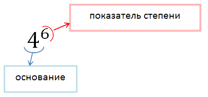
В общем виде степень с основанием «a» и
показателем «n» записывается с помощью выражения:

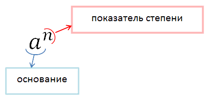
Запомните!

Степенью числа «a» с натуральным показателем «n»,
бóльшим 1, называется произведение «n»
одинаковых множителей, каждый из которых равен числу
«a».

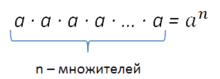
Запись «aⁿ» читается так:
«а в степени
n» или «n-ая степень числа
a».

Исключение составляют записи:

a² — её можно произносить как «а в квадрате»;
a³ — её можно произносить как «а в кубе».

Конечно, выражения выше можно читать и по определению степени:

a² — «а во второй степени»;
a³ — «а в третьей степени».

Особые случаи возникают, если показатель степени равен единице или нулю (n = 1; n = 0).

Запомните!

Степенью числа «а» с показателем n = 1 является само это число:
a¹ = a

Любое число в нулевой степени равно единице.
a⁰ = 1

Ноль в любой натуральной степени равен нулю.
0ⁿ = 0

Единица в любой степени равна 1.
1ⁿ = 1

Выражение 0⁰ (ноль в нулевой степени) считают лишённым смысла.

(−32)⁰ = 1
0²⁵³ = 0
1⁴ = 1

При решении примеров нужно помнить, что возведением в степень называется нахождение числового или буквенного значения после его возведения в
степень.

Пример. Возвести в степень.

5³ = 5 · 5 · 5 = 125
2,5² = 2,5 · 2,5 = 6,25
()⁴
=
·

·

·

=

3 · 3 · 3 · 3

4 · 4 · 4 · 4

=

Возведение в степень отрицательного числа

Основание степени (число, которое возводят в степень) может быть любым
числом — положительным, отрицательным или нулём.

Запомните!

При возведении в степень положительного числа
получается положительное число.

При возведении нуля в натуральную степень получается ноль.

При возведении в степень отрицательного числа в результате может получиться
как положительное число, так и отрицательное число. Это зависит от того чётным или
нечётным числом был показатель степени.

Рассмотрим примеры возведения в степень отрицательных чисел.

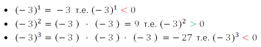
Из рассмотренных примеров видно, что если отрицательное число возводится в нечётную степень,
то получается отрицательное число. Так как произведение
нечётного количество отрицательных сомножителей отрицательно.

Если же отрицательное число возводится в чётную степень, то получается положительное число.
Так как произведение чётного количество отрицательных сомножителей положительно.

Запомните!

Отрицательное число, возведённое в
чётную степень, есть число
положительное.

Отрицательное число, возведённое в
нечётную степень, — число
отрицательное.

Квадрат любого числа есть положительное число или нуль, то есть:

a² ≥ 0 при любом a.

2 · (−3)² = 2 · (−3) · (−3) = 2 · 9 = 18
−5 · (−2)³ = −5 · (−8) = 40

Обратите внимание!

При решении примеров на возведение в степень часто делают ошибки, забывая, что записи
(−5)⁴ и
−5⁴ это разные выражения. Результаты возведения
в степень данных выражений будут разные.

Вычислить (−5)⁴ означает найти значение четвёртой степени отрицательного числа.

(−5)⁴ = (−5) · (−5) · (−5) · (−5) = 625

В то время как найти «−5⁴» означает, что пример нужно решать в 2 действия:

Возвести в четвёртую степень положительное число 5.

5⁴ = 5 · 5 · 5 · 5 = 625
Поставить перед полученным результатом знак «минус» (то есть выполнить
действие вычитание).

−5⁴ = −625

Пример. Вычислить: −6² − (−1)⁴

−6² − (−1)⁴ = −37

6² = 6 · 6 = 36
−6² = −36
(−1)⁴ = (−1) · (−1) · (−1) · (−1) = 1
−(−1)⁴ = −1
−36 − 1 = −37

Порядок действий в примерах со степенями

Вычисление значения называется действием возведения в степень. Это действие третьей ступени.

Запомните!

В выражениях со степенями, не содержащими скобки, сначала выполняют
вовзведение в степень, затем умножение и деление, а в
конце сложение и вычитание.

Если в выражении есть скобки, то сначала в указанном выше порядке выполняют действия в скобках,
а потом оставшиеся действия в том же порядке слева направо.

Пример. Вычислить:

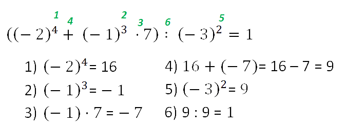
Для облегчения решения примеров полезно знать и пользоваться
таблицей степеней, которую вы можете бесплатно скачать на нашем сайте.

Для проверки своих результатов вы можете воспользоваться на нашем сайте калькулятором
«Возведение в степень онлайн».

Источник

Что такое степень?

Степенью называют произведение из нескольких одинаковых множителей. Например:

2 × 2 × 2

Значение данного выражения равно 8

2 × 2 × 2 = 8

Левую часть этого равенства можно сделать короче – сначала записать повторяющийся множитель и указать над ним сколько раз он повторяется. Повторяющийся множитель в данном случае это 2. Повторяется он три раза. Поэтому над двойкой записываем тройку:

2³ = 8

Это выражение читается так: «два в третьей степени равно восемь» или «третья степень числа 2 равна 8».

Короткую форму записи перемножения одинаковых множителей используют чаще. Поэтому надо помнить, что если над каким-то числом надписано другое число, то это есть перемножение нескольких одинаковых множителей.

Например, если дано выражение 5³, то следует иметь ввиду, что это выражение равносильно записи 5 × 5 × 5.

Число, которое повторяется называют основанием степени. В выражении 5³основанием степени является число 5.

А число, которое надписано над числом 5 называют показателем степени. В выражении 5³показателем степени является число 3. Показатель степени показывает сколько раз повторяется основание степени. В нашем случае основание 5 повторяется три раза

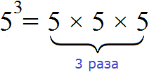
Саму операцию перемножения одинаковых множителей называют возведением в степень.

Например, если нужно найти произведение из четырёх одинаковых множителей, каждый из которых равен 2, то говорят, что число 2 возводится в четвёртую степень:

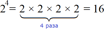
Видим, что число 2 в четвёртой степени есть число 16.

Отметим, что в данном уроке мы рассматриваем степени с натуральным показателем. Это вид степени, показателем которой является натуральное число. Напомним, что натуральными называют целые числа, которые больше нуля. Например, 1, 2, 3 и так далее.

Вообще, определение степени с натуральным показателем выглядит следующим образом:

Степень числа a с натуральным показателем n — это выражение вида aⁿ, которое равно произведению n множителей, каждый из которых равен a

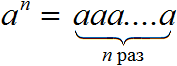
Примеры:

Следует быть внимательным при возведении числа в степень. Часто по невнимательности человек умножает основание степени на показатель.

Например, число 5 во второй степени есть произведение двух множителей каждый из которых равен 5. Это произведение равно 25

Теперь представим, что мы по невнимательности умножили основание 5 на показатель 2

Получилась ошибка, поскольку число 5 во второй степени не равно 10.

Дополнительно следует упомянуть, что степень числа с показателем 1, есть само это число:

Например, число 5 в первой степени есть само число 5

Соответственно, если у числа отсутствует показатель, то надо считать, что показатель равен единице.

Например, числа 1, 2, 3 даны без показателя, поэтому их показатели будут равны единице. Каждое из этих чисел можно записать с показателем 1

А если возвести 0 в какую-нибудь степень, то получится 0. Действительно, сколько бы раз ничего не умножалось на само себя получится ничего. Примеры:

А выражение 0⁰ не имеет смысла. Но в некоторых разделах математики, в частности анализе и теории множеств, выражение 0⁰ может иметь смысл.

Для тренировки решим несколько примеров на возведение чисел в степени.

Пример 1. Возвести число 3 во вторую степень.

Число 3 во второй степени это произведение двух множителей, каждый из которых равен 3

3² = 3 × 3 = 9

Пример 2. Возвести число 2 в четвертую степень.

Число 2 в четвертой степени это произведение четырёх множителей, каждый из которых равен 2

2⁴ =2 × 2 × 2 × 2 = 16

Пример 3. Возвести число 2 в третью степень.

Число 2 в третьей степени это произведение трёх множителей, каждый из которых равен 2

2³ =2 × 2 × 2 = 8

Возведение в степень числа 10

Чтобы возвести в степень число 10, достаточно дописать после единицы количество нулей, равное показателю степени.

Например, возведем число 10 во вторую степень. Сначала запишем само число 10 и в качестве показателя укажем число 2

10²

Теперь ставим знак равенства, записываем единицу и после этой единицы записываем два нуля, поскольку количество нулей должно быть равно показателю степени

10² = 100

Значит, число 10 во второй степени это число 100. Связано это с тем, что число 10 во второй степени это произведение двух множителей, каждый из которых равен 10

10² = 10 × 10 = 100

Пример 2. Возведём число 10 в третью степень.

В данном случае после единицы будут стоять три нуля:

10³ = 1000

Пример 3. Возведем число 10 в четвёртую степень.

В данном случае после единицы будут стоять четыре нуля:

10⁴ = 10000

Пример 4. Возведем число 10 в первую степень.

В данном случае после единицы будет стоять один нуль:

10¹ = 10

Представление чисел 10, 100, 1000 в виде степени с основанием 10

Чтобы представить числа 10, 100, 1000 и 10000 в виде степени с основанием 10, нужно записать основание 10, и в качестве показателя указать число, равное количеству нулей исходного числа.

Представим число 10 в виде степени с основанием 10. Видим, что в нём один нуль. Значит, число 10 в виде степени с основанием 10 будет представлено как 10¹

10 = 10¹

Пример 2. Представим число 100 в виде степени основанием 10. Видим, что число 100 содержит два нуля. Значит, число 100 в виде степени с основанием 10 будет представлено как 10²

100 = 10²

Пример 3. Представим число 1 000 в виде степени с основанием 10.

1 000 = 10³

Пример 4. Представим число 10 000 в виде степени с основанием 10.

10 000 = 10⁴

Возведение в степень отрицательного числа

При возведении в степень отрицательного числа, его обязательно нужно заключить в скобки.

Например, возведём отрицательное число −2 во вторую степень. Число −2 во второй степени это произведение двух множителей, каждый из которых равен (−2)

(−2)² = (−2) × (−2) = 4

Если бы мы не заключили в скобки число −2, то получилось бы что мы вычисляем выражение −2², которое не равно 4. Выражение −2² будет равно −4. Чтобы понять почему, коснёмся некоторых моментов.

Когда мы ставим перед положительным числом минус, мы тем самым выполняем операцию взятия противоположного значения.

Допустим, дано число 2, и нужно найти его противоположное число. Мы знаем, что противоположное числу 2 это число −2. Иными словами, чтобы найти противоположное число для 2, достаточно поставить минус перед этим числом. Вставка минуса перед числом уже считается в математике полноценной операцией. Эту операцию, как было указано выше, называют операцией взятия противоположного значения.

В случае с выражением −2² происходит две операции: операция взятия противоположного значения и возведение в степень. Возведение в степень является более приоритетной операцией, чем взятие противоположного значения.

Поэтому выражение −2² вычисляется в два этапа. Сначала выполняется операция возведения в степень. В данном случае во вторую степень было возведено положительное число 2

Затем выполнилось взятие противоположного значения. Это противоположное значение было найдено для значения 4. А противоположное значение для 4 это −4

−2² = −4

Скобки же имеют самый высокий приоритет выполнения. Поэтому в случае вычисления выражения (−2)² сначала выполняется взятие противоположного значения, а затем во вторую степень возводится отрицательное число −2. В результате получается положительный ответ 4, поскольку произведение отрицательных чисел есть положительное число.

Пример 2. Возвести число −2 в третью степень.

Число −2 в третьей степени это произведение трёх множителей, каждый из которых равен (−2)

(−2)³ = (−2) × (−2) × (−2) = −8

Пример 3. Возвести число −2 в четвёртую степень.

Число −2 в четвёртой степени это произведение четырёх множителей, каждый из которых равен (−2)

(−2)⁴ = (−2) × (−2) × (−2) × (−2) = 16

Легко заметить, что при возведении в степень отрицательного числа может получиться либо положительный ответ либо отрицательный. Знак ответа зависит от показателя исходной степени.

Если показатель степени чётный, то ответ будет положительным. Если показатель степени нечётный, ответ будет отрицательным. Покажем это на примере числа −3

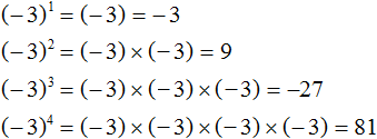
В первом и в третьем случае показатель был нечётным числом, поэтому ответ стал отрицательным.

Во втором и в четвёртом случае показатель был чётным числом, поэтому ответ стал положительным.

Пример 7. Возвести число −5 в третью степень.

Число −5 в третьей степени это произведение трёх множителей каждый из которых равен −5. Показатель 3 является нечётным числом, поэтому мы заранее можем сказать, что ответ будет отрицательным:

(−5)³ = (−5) × (−5) × (−5) = −125

Пример 8. Возвести число −4 в четвёртую степень.

Число −4 в четвёртой степени это произведение четырёх множителей, каждый из которых равен −4. При этом показатель 4 является чётным, поэтому мы заранее можем сказать, что ответ будет положительным:

(−4)⁴ = (−4) × (−4) × (−4) × (−4) = 256

Нахождение значений выражений

При нахождении значений выражений, не содержащих скобки, возведение в степень будет выполняться в первую очередь, далее умножение и деление в порядке их следования, а затем сложение и вычитание в порядке их следования.

Пример 1. Найти значение выражения 2 + 5²

Сначала выполняется возведение в степень. В данном случае во вторую степень возводится число 5 — получается 25. Затем этот результат складывается с числом 2

2 + 5² = 2 + 25 = 27

Пример 10. Найти значение выражения −6² × (−12)

Сначала выполняется возведение в степень. Заметим, что число −6 не взято в скобки, поэтому во вторую степень будет возведено число 6, затем перед результатом будет поставлен минус:

−6² × (−12) = −36 × (−12)

Завершаем пример, умножив −36 на (−12)

−6² × (−12) = −36 × (−12) = 432

Пример 11. Найти значение выражения −3 × 2²

Сначала выполняется возведение в степень. Затем полученный результат перемножается с числом −3

−3 × 2² = −3 × 4 = −12

Если выражение содержит скобки, то сначала нужно выполнить действия в этих скобках, далее возведение в степень, затем умножение и деление, а затем сложение и вычитание.

Пример 12. Найти значение выражения (3² + 1 × 3) − 15 + 5

Сначала выполняем действия в скобках. Внутри скобок применяем ранее изученные правила, а именно сначала возводим во вторую степень число 3, затем выполняем умножение 1 × 3, затем складываем результаты возведения в степень числа 3 и умножения 1 × 3. Далее выполняется вычитание и сложение в порядке их следования. Расставим такой порядок выполнения действия над исходным выражением:

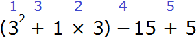
(3² + 1 × 3) − 15 + 5 = 12 − 15 + 5 = 2

Пример 13. Найти значение выражения 2 × 5³ + 5 × 2³

Сначала возведем числа в степени, затем выполним умножение и сложим полученные результаты:

2 × 5³ + 5 × 2³ = 2 × 125 + 5 × 8 = 250 + 40 = 290

Тождественные преобразования степеней

Над степенями можно выполнять различные тождественные преобразования, тем самым упрощая их.

Допустим, потребовалось вычислить выражение (2³)². В данном примере два в третьей степени возводится во вторую степень. Иными словами, степень возводится в другую степень.

(2³)² это произведение двух степеней, каждая из которых равна 2³

При этом каждая из этих степеней является произведением трёх множителей, каждый из которых равен 2

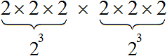
Получили произведение 2 × 2 × 2 × 2 × 2 × 2, которое равно 64. Значит значение выражения (2³)² или равно 64

Этот пример можно значительно упростить. Для этого показатели выражения (2³)² можно перемножить и записать это произведение над основанием 2

Получили 2⁶. Два в шестой степени это произведение шести множителей, каждый из которых равен 2. Это произведение равно 64

Данное свойство работает по причине того, что 2³ это произведение 2 × 2 × 2, которое в свою очередь повторяется два раза. Тогда получается, что основание 2 повторяется шесть раз. Отсюда можно записать, что 2 × 2 × 2 × 2 × 2 × 2 это 2⁶

Вообще, для любого основания a с показателями m и n, выполняется следующее равенство:

(aⁿ)^m = a^n × m

Это тождественное преобразование называют возведением степени в степень. Его можно прочитать так: «При возведении степени в степень основание оставляют без изменений, а показатели перемножают».

После перемножения показателей, получится другая степень, значение которой можно найти.

Пример 2. Найти значение выражения (3²)²

В данном примере основанием является 3, а числа 2 и 2 являются показателями. Воспользуемся правилом возведения степени в степень. Основание оставим без изменений, а показатели перемножим:

Получили 3⁴. А число 3 в четвёртой степени есть 81

Рассмотрим остальные преобразования.

Умножение степеней

Чтобы перемножить степени, нужно по отдельности вычислить каждую степень, и полученные результаты перемножить.

Например, умножим 2² на 3³.

2² это число 4, а 3³ это число 27. Перемножаем числа 4 и 27, получаем 108

2² × 3³ = 4 × 27 = 108

В этом примере основания степеней были разными. В случае, если основания будут одинаковыми, то можно записать одно основание, а в качестве показателя записать сумму показателей исходных степеней.

Например, умножим 2² на 2³

В данном примере основания у степеней одинаковые. В этом случае можно записать одно основание 2 и в качестве показателя записать сумму показателей степеней 2² и 2³. Иными словами, основание оставить без изменений, а показатели исходных степеней сложить. Выглядеть это будет так:

Получили 2⁵. Число 2 в пятой степени есть 32

Данное свойство работает по причине того, что 2² это произведение 2 × 2, а 2³ это произведение 2 × 2 × 2. Тогда получается произведение из пяти одинаковых множителей, каждый из которых равен 2. Это произведение представимо в виде 2⁵

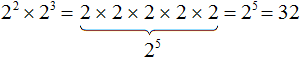
Вообще, для любого a и показателей m и n выполняется следующее равенство:

Это тождественное преобразование носит название основного свойства степени. Его можно прочитать так: «При перемножении степеней с одинаковыми основаниями, основание оставляют без изменений, а показатели складывают».

Отметим, что данное преобразование можно применять при любом количестве степеней. Главное, чтобы основание было одинаковым.

Например, найдем значение выражения 2¹ × 2² × 2³. Основание 2 оставим без изменений, а показатели сложим:

В некоторых задачах достаточным бывает выполнить соответствующее преобразование, не вычисляя итоговую степень. Это конечно же очень удобно, поскольку вычислять большие степени не так-то просто.

Пример 1. Представить в виде степени выражение 5⁸ × 25

В данной задаче нужно сделать так, чтобы вместо выражения 5⁸ × 25 получилась одна степень.

Число 25 можно представить в виде 5². Тогда получим следующее выражение:

В этом выражении можно применить основное свойство степени — основание 5 оставить без изменений, а показатели 8 и 2 сложить:

Задачу можно считать решённой, поскольку мы представили выражение 5⁸ × 25 в виде одной степени, а именно в виде степени 5¹⁰.

Запишем решение покороче:

Пример 2. Представить в виде степени выражение 2⁹ × 32

Число 32 можно представить в виде 2⁵. Тогда получим выражение 2⁹ × 2⁵. Далее можно применить основание свойство степени — основание 2 оставить без изменений, а показатели 9 и 5 сложить. В результате получится следующее решение:

Пример 3. Вычислите произведение 3 × 3, используя основное свойство степени.

Все хорошо знают, что три умножить на три равно девять, но задача требует в ходе решения воспользоваться основным свойством степени. Как это сделать?

Вспоминаем, что если число дано без показателя, то показатель нужно считать равным единице. Стало быть сомножители 3 и 3 можно записать в виде 3¹ и 3¹

3¹ × 3¹

Теперь воспользуемся основным свойством степени. Основание 3 оставляем без изменений, а показатели 1 и 1 складываем:

3¹ × 3¹ = 3²

Далее вычисляем значение выражения. Число 3 во второй степени равно числу 9

3¹ × 3¹ = 3² = 9

Пример 4. Вычислите произведение 2 × 2 × 3² × 3³, используя основное свойство степени.

Произведение 2 × 2 заменим на 2¹ × 2¹, затем на 2^1 + 1, а затем на 2². Произведение 3² × 3³ заменим на 3^2 + 3, а затем на 3⁵

Далее вычисляем значение каждой степени и находим произведение:

Пример 5. Выполнить умножение x × x

Это два одинаковых буквенных сомножителя с показателями 1. Для наглядности запишем эти показатели. Далее основание x оставим без изменений, а показатели сложим:

Находясь у доски, не следует записывать перемножение степеней с одинаковыми основаниями так подробно, как это сделано здесь. Такие вычисления нужно выполнять в уме. Подробная запись скорее всего будет раздражать учителя и он снизит за это оценку. Здесь же подробная запись дана, чтобы материал был максимально доступным для понимания.

Решение данного примера желательно записать так:

Пример 6. Выполнить умножение x² × x

Показатель второго сомножителя равен единице. Для наглядности запишем его. Далее основание оставим без изменений, а показатели сложим:

Пример 7. Выполнить умножение y³y²y

Показатель третьего сомножителя равен единице. Для наглядности запишем его. Далее основание оставим без изменений, а показатели сложим:

Пример 8. Выполнить умножение aa³a²a⁵

Показатель первого сомножителя равен единице. Для наглядности запишем его. Далее основание оставим без изменений, а показатели сложим:

Пример 9. Представить степень 3⁸ в виде произведения степеней с одинаковыми основаниями.

В данной задаче нужно составить произведение степеней, основания которых будут равны 3, и сумма показателей которых будет равна 8. Можно использовать любые показатели. Представим степень 3⁸ в виде произведения степеней 3⁵ и 3³

В данном примере мы опять же опирались на основное свойство степени. Ведь выражение 3⁵ × 3³ можно записать как 3^5 + 3, откуда 3⁸.

Конечно можно было представить степень 3⁸ в виде произведения других степеней. Например, в виде 3⁷ × 3¹, поскольку это произведение тоже равно 3⁸

Представление степени в виде произведения степеней с одинаковыми основаниями это по большей части творческая работа. Поэтому не нужно бояться экспериментировать.

Пример 10. Представить степень x¹² в виде различных произведений степеней с основаниями x.

Воспользуемся основным свойство степени. Представим x¹² в виде произведений с основаниями x, и сумма показателей которых равна 12

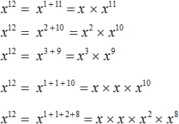
Конструкции с суммами показателей были записаны для наглядности. Чаще всего их можно пропустить. Тогда получится компактное решение:

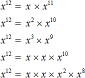
Возведение в степень произведения

Чтобы возвести в степень произведение, нужно возвести в указанную степень каждый множитель этого произведения и перемножить полученные результаты.

Например, возведём во вторую степень произведение 2 × 3. Возьмём в скобки данное произведение и в качестве показателя укажем 2

Теперь возведём во вторую степень каждый множитель произведения 2 × 3 и перемножим полученные результаты:

Принцип работы данного правила основан на определении степени, которое было дано в самом начале.

Возвести произведение 2 × 3 во вторую степень означает повторить данное произведение два раза. А если повторить его два раза, то можно получить следующее:

2 × 3 × 2 × 3

От перестановки мест сомножителей произведение не меняется. Это позволяет сгруппировать одинаковые множители:

2 × 2 × 3 × 3

Повторяющиеся множители можно заменить на короткие записи — основания с показателями. Произведение 2 × 2 можно заменить на 2², а произведение 3 × 3 можно заменить на 3². Тогда выражение 2 × 2 × 3 × 3 обращается в выражение 2² × 3².

Пусть ab исходное произведение. Чтобы возвести данное произведение в степень n, нужно по отдельности возвести множители a и b в указанную степень n

Данное свойство справедливо для любого количества множителей. Следующие выражения также справедливы:

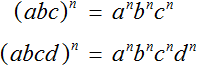
Пример 2. Найти значение выражения (2 × 3 × 4)²

В данном примере нужно возвести во вторую степень произведение 2 × 3 × 4. Чтобы сделать это, нужно возвести во вторую степень каждый множитель этого произведения и перемножить полученные результаты:

Пример 3. Возвести в третью степень произведение a × b × c

Заключим в скобки данное произведение, и в качестве показателя укажем число 3

Далее возводим в третью степень каждый множитель данного произведения:

Пример 4. Возвести в третью степень произведение 3xyz

Заключим в скобки данное произведение, и в качестве показателя укажем 3

(3xyz)³

Возведём в третью степень каждый множитель данного произведения:

(3xyz)³ = 3³x³y³z³

Число 3 в третьей степени равно числу 27. Остальное оставим без изменений:

(3xyz)³ = 3³x³y³z³ = 27x³y³z³

В некоторых примерах умножение степеней с одинаковыми показателями можно заменять на произведение оснований с одним показателем.

Например, вычислим значение выражения 5² × 3². Возведем каждое число во вторую степень и перемножим полученные результаты:

5² × 3² = 25 × 9 = 225

Но можно не вычислять по отдельности каждую степень. Вместо этого, данное произведение степеней можно заменить на произведение с одним показателем (5 × 3)². Далее вычислить значение в скобках и возвести полученный результат во вторую степень:

5² × 3² = (5 × 3)² = (15)² = 225

В данном случае опять же было использовано правило возведения в степень произведения. Ведь, если (a × b)ⁿ = aⁿ × bⁿ, то aⁿ × bⁿ= (a × b)ⁿ. То есть левая и правая часть равенства поменялись местами.

Возведение степени в степень

Это преобразование мы рассматривали в качестве примера, когда пытались понять суть тождественных преобразований степеней.

При возведении степени в степень основание оставляют без изменений, а показатели перемножают:

(aⁿ)^m = a^n × m

К примеру, выражение (2³)² является возведением степени в степень — два в третьей степени возводится во вторую степень. Чтобы найти значение этого выражения, основание можно оставить без изменений, а показатели перемножить:

(2³)² = 2^3 × 2 = 2⁶

Далее вычислить степень 2⁶, которая равна 64

(2³)² = 2^3 × 2 = 2⁶ = 64

Данное правило основано на предыдущих правилах: возведении в степень произведения и основного свойства степени.

Вернёмся к выражению (2³)². Выражение в скобках 2³ представляет собой произведение из трёх одинаковых множителей, каждый из которых равен 2. Тогда в выражении (2³)² степень, находящуюся внутри скобок можно заменить на произведение 2 × 2 × 2.

(2 × 2 × 2)²

А это есть возведение в степень произведения, которое мы изучили ранее. Напомним, что для возведения в степень произведения, нужно возвести в указанную степень каждый множитель данного произведения и полученные результаты перемножить:

(2 × 2 × 2)² = 2² × 2² × 2²

Теперь имеем дело с основным свойством степени. Основание оставляем без изменений, а показатели складываем:

(2 × 2 × 2)² = 2² × 2² × 2² = 2^{2 + 2 + 2} = 2⁶

Как и раньше получили 2⁶. Значение этой степени равно 64

(2 × 2 × 2)² = 2² × 2² × 2² = 2^{2 + 2 + 2} = 2⁶ = 64

В степень также может возводиться произведение, сомножители которого тоже являются степенями.

Например, найдём значение выражения (2² × 3²)³. Здесь показатели каждого множителя нужно умножить на общий показатель 3. Далее найти значение каждой степени и вычислить произведение:

(2² × 3²)³= 2^2×3 × 3^2×3 = 2⁶× 3⁶ = 64 × 729 = 46656

Примерно тоже самое происходит при возведении в степени произведения. Мы говорили, что при возведении в степень произведения, в указанную степень возводится каждый множитель этого произведения.

Например, чтобы возвести произведение 2 × 4 в третью степень, нужно записать следующее выражение:

Но ранее было сказано, что если число дано без показателя, то показатель надо считать равным единице. Получается, что множители произведения 2 × 4 изначально имеют показатели равные 1. Значит в третью степень возводилось выражение 2¹ × 4¹. А это есть возведение степени в степень.

Перепишем решение с помощью правила возведения степени в степень. У нас должен получиться тот же результат:

Пример 2. Найти значение выражения (3³)²

Основание оставляем без изменений, а показатели перемножаем:

Получили 3⁶. Число 3 в шестой степени есть число 729

Пример 3. Выполнить возведение в степень в выражении (xy)³

Возведём в третью степень каждый множитель произведения:

Пример 4. Выполнить возведение в степень в выражении (abc)⁵

Возведём в пятую степень каждый множитель произведения:

Пример 5. Выполнить возведение в степень в выражении (−2ax)³

Возведём в третью степень каждый множитель произведения:

Поскольку в третью степень возводилось отрицательное число −2, оно было взято в скобки.

Далее нужно вычислить то, что вычисляется. В данном случае можно вычислить (−2)³ — получится −8. Буквенная часть останется без изменений:

Пример 6. Выполнить возведение в степень в выражении (10xy)²

Пример 7. Выполнить возведение в степень в выражении (−5x)³

Пример 8. Выполнить возведение в степень в выражении (−3y)⁴

Пример 9. Выполнить возведение в степень в выражении (−2abx)⁴

Пример 10. Упростите выражение x⁵ × (x²)³

Степень x⁵ пока оставим без изменений, а в выражении (x²)³ выполним возведение степени в степени:

x⁵ × (x²)³ = x⁵ × x^2 × 3 = x⁵ × x⁶

Теперь выполним умножение x⁵× x⁶. Для этого воспользуемся основным свойством степени — основание x оставим без изменений, а показатели сложим:

x⁵ × (x²)³ = x⁵ × x^2× 3 = x⁵ × x⁶ = x^5 + 6 = x¹¹

Пример 9. Найти значение выражения 4³ × 2², используя основное свойство степени.

Основное свойство степени можно использовать в случае, если основания исходных степеней одинаковы. В данном примере основания разные, поэтому для начала исходное выражение нужно немного видоизменить, а именно сделать так, чтобы основания степеней стали одинаковыми.

Посмотрим внимательно на степень 4³. Основание у этой степени есть число 4, которое можно представить в виде 2². Тогда исходное выражение примет вид (2²)³ × 2². Выполнив возведение степени в степень в выражении (2²)³, мы получим 2⁶. Тогда исходное выражение примет вид 2⁶ × 2², вычислить которое можно, используя основное свойство степени.

Запишем решение данного примера:

Деление степеней

Чтобы выполнить деление степеней, нужно найти значение каждой степени, затем выполнить деление обыкновенных чисел.

Например, разделим 4³ на 2².

Вычислим 4³, получим 64. Вычислим 2², получим 4. Теперь разделим 64 на 4, получим 16

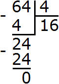
Если при делении степеней основания окажутся одинаковыми, то основание можно оставить без изменений, а из показателя степени делимого вычесть показатель степени делителя.

Например, найдем значение выражения 2³ : 2²

Основание 2 оставим без изменений, а из показателя степени делимого вычтем показатель степени делителя:

Значит, значение выражения 2³ : 2² равно 2.

Данное свойство основано на умножении степеней с одинаковыми основаниями, или как мы привыкли говорить на основном свойстве степени.

Вернемся к предыдущему примеру 2³ : 2². Здесь делимое это 2³, а делитель 2².

Разделить одно число на другое означает найти такое число, которое при умножении на делитель даст в результате делимое.

В нашем случае, разделить 2³ на 2² означает найти такую степень, которая при умножении на делитель 2² даст в результате 2³. А какую степень можно умножить на 2², чтобы получить 2³ ? Очевидно, что только степень 2¹. Из основного свойства степени имеем:

Убедиться, что значение выражения 2³ : 2² равно 2¹ можно непосредственно вычислив само выражение 2³ : 2². Для этого сначала найдём значение степени 2³, получим 8. Затем найдём значение степени 2², получим 4. Разделим 8 на 4, получим 2 или 2¹, поскольку 2 = 2¹.

2³ : 2² = 8 : 4 = 2

Таким образом, при делении степеней с одинаковыми основаниями выполняется следующее равенство:

Может случиться и так, что одинаковыми могут оказаться не только основания, но и показатели. В этом случае в ответе получится единица.

Например, найдём значение выражения 2² : 2². Вычислим значение каждой степени и выполним деление получившихся чисел:

При решении примера 2² : 2² также можно применить правило деления степеней с одинаковыми основаниями. В результате получается число в нулевой степени, поскольку разность показателей степеней 2² и 2² равна нулю:

В математике принято считать, что любое число в нулевой степени есть единица:

Почему число 2 в нулевой степени равно единице мы выяснили выше. Если вычислить 2² : 2² обычным методом, не используя правило деления степеней, получится единица.

Пример 2. Найти значение выражения 4¹² : 4¹⁰

Воспользуемся правилом деления степеней. Основание 4 оставим без изменений, а из показателя степени делимого вычтем показатель степени делителя:

4¹² : 4¹⁰ = 4^{12 − 10} = 4² = 16

Пример 3. Представить частное x³ : x в виде степени с основанием x

Воспользуемся правилом деления степеней. Основание x оставим без изменений, а из показателя степени делимого вычтем показатель степени делителя. Показатель делителя равен единице. Для наглядности запишем его:

Пример 4. Представить частное x³ : x² в виде степени с основанием x

Воспользуемся правилом деления степеней. Основание x оставим без изменений, а из показателя степени делимого вычтем показатель степени делителя:

Деление степеней можно записывать в виде дроби. Так, предыдущий пример можно записать следующим образом:

Числитель и знаменатель дроби разрешается записывать в развёрнутом виде, а именно в виде произведений одинаковых множителей. Степень x³ можно записать как x × x × x, а степень x² как x × x. Тогда конструкцию x^3 − 2 можно будет пропустить и воспользоваться сокращением дроби. В числителе и в знаменателе можно будет сократить по два множителя x. В результате останется один множитель x

Или ещё короче:

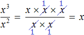
Также, полезно уметь быстро сокращать дроби, состоящие из степеней. Например, дробь можно сократить на x². Чтобы сократить дробь на x² нужно числитель и знаменатель дроби разделить на x²

Деление степеней подробно можно не расписывать. Приведённое сокращение можно выполнить короче:

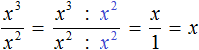
Или ещё короче:

Пример 5. Выполнить деление x¹² : x³

Запишем решение при помощи сокращения дроби. Деление степеней x¹² : x³ запишем в виде . Далее сократим данную дробь на x³.

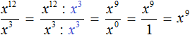
Пример 6. Найти значение выражения

В числителе выполним умножение степеней с одинаковыми основаниями:

Теперь применяем правило деления степеней с одинаковыми основаниями. Основание 7 оставляем без изменений, а из показателя степени делимого вычтем показатель степени делителя:

Завершаем пример, вычислив степень 7²

Пример 7. Найти значение выражения

Выполним в числителе возведение степени в степень. Сделать это нужно с выражением (2³)⁴

Теперь выполним в числителе умножение степеней с одинаковыми основаниями:

Теперь применяем правило деления степеней с одинаковыми основаниями:

Значит, значение выражения равно 16

В некоторых примерах можно сокращать одинаковые множители в ходе решения. Это позволяет упростить выражение и само вычисление в целом.

Например, найдём значение выражения . Степень 4³ запишем в виде возведения степени в степень (2²)³. Тогда получим следующее выражение:

В числителе выполним возведение степени в степень. Сделать это нужно с выражением (2²)³

В числителе и в знаменателе получившегося выражения содержится степень 2⁶, которую можно сократить на 2⁶

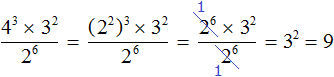
Видим, что в результате осталась единственная степень 3², значение которой равно 9.

Пример 8. Найти значение выражения

В знаменателе содержится произведение степеней с одинаковыми показателями. Согласно правилу возведения в степень произведения, конструкцию 7⁵ × 4⁵ можно представить в виде степени с одним показателем (7 × 4)⁵. Далее перемножим выражение в скобках, получим 28⁵. В результате исходное выражение примет следующий вид:

Теперь можно применить правило деления степеней:

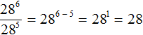
Значит, значение выражения равно 28. Запишем решение полностью:

Возведение в степень обыкновенных дробей

Чтобы возвести в степень обыкновенную дробь, нужно возвести в указанную степень числитель и знаменатель этой дроби.

Например, возведём обыкновенную дробь во вторую степень. Возьмём в скобки данную дробь и в качестве показателя укажем 2

Если не брать в скобки всю дробь, то это равносильно возведению в степень только числителя данной дроби. Иными словами, если мы хотим возвести во вторую степень дробь , мы не должны записывать это как .

Итак, чтобы вычислить значение выражения , нужно возвести во вторую степень числитель и знаменатель данной дроби:

Получили дробь в числителе и в знаменателе которой содержатся степени. Вычислим каждую степень по отдельности

Значит обыкновенная дробь во второй степени равна дроби .

Приведённое правило работает следующим образом. Дробь во второй степень это произведение двух дробей, каждая из которых равна

Мы помним, что для перемножения дробей необходимо перемножить их числители и знаменатели:

А поскольку в числителе и в знаменателе происходит перемножение одинаковых множителей, то выражения 2 × 2 и 3 × 3 можно заменить на 2² и 3² соответственно:

Откуда и получится ответ .

Вообще, для любого a и b ≠ 0 выполняется следующее равенство:

Это тождественное преобразование называют возведением в степень обыкновенной дроби.

Пример 2. Возвести дробь в третью степень

Заключим данную дробь в скобки и в качестве показателя укажем число 3. Далее возведём числитель и знаменатель данной дроби в третью степень и вычислим получившуюся дробь:

Отрицательная дробь возводится в степень таким же образом, но перед вычислениями надо определиться какой знак будет иметь ответ. Если показатель четный, то ответ будет положительным. Если показатель нечетный, то ответ будет отрицательным.

Например, возведём дробь во вторую степень:

Показатель является чётным числом. Значит ответ будет положительным. Далее применяем правило возведения в степень дроби и вычисляем получившуюся дробь:

Ответ положителен по причине того, что выражение представляет собой произведение двух сомножителей, каждый из которых равен дроби

А произведение отрицательных чисел (в том числе и рациональных) есть положительное число:

Если возводить дробь в третью степень, то ответ будет отрицательным, поскольку в данном случае показатель будет нечётным числом. Правило возведения в степень остаётся тем же, но перед выполнением этого возведения, нужно будет поставить минус:

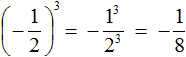
Здесь ответ отрицателем по причине того, что выражение представляет собой произведение трёх множителей, каждый из которых равен дроби

Сначала перемножили и , получили , но затем умножив на мы получим отрицательный ответ

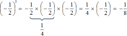
Пример 3. Найти значение выражения

Выполним возведение в степень обыкновенной дроби:

Далее вычислим значение получившегося выражения:

Возведение в степень десятичных дробей

При возведении в степень десятичной дроби её необходимо заключить в скобки. Например, возведём во вторую степень десятичную дробь 1,5

Допускается переводить десятичную дробь в обыкновенную и возводить в степень эту обыкновенную дробь. Решим предыдущий пример, переведя десятичную дробь в обыкновенную:

Пример 2. Найти значение степени (−1,5)³

Показатель степени является нечётным числом. Значит ответ будет отрицательным

Пример 3. Найти значение степени (−2,4)²

Показатель степени является чётным числом. Значит ответ будет положительным:

Задания для самостоятельного решения

Задание 1. Найдите значение выражения:

Решение:

Задание 2. Найдите значение выражения:

Решение:

Задание 3. Найдите значение выражения:

Решение:

Задание 4. Найдите значение выражения:

Решение:

Задание 5. Найдите значение выражения:

Решение:

Задание 6. Найдите значение выражения:

Решение:

Задание 7. Представьте в виде степени произведение:

Решение:

Задание 8. Представьте в виде степени произведение:

Решение:

Задание 9. Представьте в виде степени произведение:

Решение:

Задание 10. Представьте в виде степени произведение:

Решение:

Задание 11. Представьте в виде степени произведение:

Решение:

Задание 12. Представьте в виде степени произведение:

Решение:

Задание 13. Представьте в виде степени частное:

Решение:

Задание 14. Представьте в виде степени частное:

Решение:

Задание 15. Представьте в виде степени частное:

Решение:

Задание 16. Представьте в виде степени частное:

Решение:

Задание 17. Представьте в виде степени частное:

Решение:

Задание 18. Представьте в виде степени частное и найдите значение получившейся степени при x = 3 и n = 2

Решение:

Задание 19. Представьте в виде степени частное:

Решение:

Задание 20. Сократите дробь на c¹

Решение:

Задание 21. Представьте в виде степени следующее произведение:

Решение:

Задание 22. Представьте в виде степени следующее произведение:

Решение:

Задание 23. Представьте в виде степени следующее произведение:

Решение:

Задание 24. Представьте в виде степени следующее произведение:

Решение:

Задание 25. Представьте в виде степени следующее произведение:

Решение:

Задание 26. Представьте следующую степень в виде произведения степеней:

Решение:

Задание 27. Представьте следующую степень в виде произведения степеней:

Решение:

Задание 28. Представьте следующую степень в виде произведения степеней:

Решение:

Задание 29. Пользуясь тождественными преобразованиями степеней, найдите значение следующего выражения:

Решение:

Задание 30. Пользуясь тождественными преобразованиями степеней, найдите значение следующего выражения:

Решение:

Задание 31. Пользуясь тождественными преобразованиями степеней, найдите значение следующего выражения:

Решение:

Задание 32. Представьте в виде степени следующее выражение:

Решение:

Задание 33. Представьте в виде степени следующее выражение:

Решение:

Задание 34. Представьте в виде степени следующее выражение:

Решение:

Задание 35. Представьте в виде степени следующее выражение:

Решение:

Задание 36. Представьте в виде степени следующее выражение:

Решение:

Задание 37. Представьте в виде степени следующее выражение:

Решение:

Задание 38. Найдите значение следующего выражения:

Решение:

Задание 39. Найдите значение следующего выражения:

Решение:

Задание 40. Найдите значение следующего выражения:

Решение:

Задание 41. Найдите значение следующего выражения:

Решение:

Задание 42. Найдите значение следующего выражения:

Решение:

Задание 43. Найдите значение следующего выражения:

Решение:

Задание 44. Найдите значение следующего выражения:

Решение:

Понравился урок?
Вступай в нашу новую группу Вконтакте и начни получать уведомления о новых уроках

Возникло желание поддержать проект?
Используй кнопку ниже

Источник

Возведение в степень – это такая же математическая операция, как сложение, вычитание, умножение или деление.

Сейчас объясню все человеческим языком на очень простых примерах. Будь внимателен. Примеры элементарные, но объясняющий важные вещи. Начнем со сложения.

Сложение

( 2+2+2+2+2+2+2+2=16 )

Объяснять тут нечего. Ты и так все знаешь: нас восемь человек. У каждого по две бутылки колы. Сколько всего колы? Правильно – 16 бутылок. Теперь умножение.

Умножение

Тот же самый пример с колой можно записать по-другому: (displaystyle 2cdot 8=16).

Математики – люди хитрые и ленивые. Они сначала замечают какие-то закономерности, а потом придумывают способ как быстрее их «считать».

В нашем случае они заметили, что у каждого из восьми человек одинаковое количество бутылок колы и придумали прием, который называется умножением.

Согласись, (displaystyle 2cdot 8=16) считается легче и быстрее, чем (displaystyle 2+2+2+2+2+2+2+2=16).

И еще одна важная деталь. Ошибок при таком счете делается гораздо меньше. Математики из Стэнфорда, кстати, считают, что человек, знающий приемы счета, делает это в два раза легче и быстрее и совершает в два раза меньше ошибок. Работы меньше, а результат лучше.

Круто, да?

Итак, чтобы считать быстрее, легче и без ошибок, нужно всего лишь запомнить таблицу умножения. Ты, конечно, можешь делать все медленнее, труднее и с ошибками, но лучше ее запомнить! Вот таблица умножения. Выучи ее наизусть.

И другая таблица, красивее:

А какие еще хитрые приемы счета придумали ленивые математики? Правильно – возведение числа в степень.

Возведение числа в степень

Если тебе нужно умножить число само на себя пять раз, то математики говорят, что тебе нужно возвести это число в пятую степень.

Например, (displaystyle 2cdot 2cdot 2cdot 2cdot 2={{2}^{5}}). Математики помнят, что два в пятой степени – это (displaystyle 32).

И решают такие задачки в уме – быстрее, легче и без ошибок.

Для этого нужно всего лишь запомнить то, что выделено цветом в таблице степеней чисел. Поверь, это сильно облегчит тебе жизнь.

Кстати, почему вторую степень называют квадратом числа, а третью – кубом? Что это значит? Очень хороший вопрос. Сейчас будут тебе и квадраты, и кубы.

Примеры из жизни

Далее, почему говорят «степень числа с натуральным показателем»?

Ты уже наверное, догадался: потому что показатель степени – это натуральное число. Да, но что такое натуральное число? Элементарно! Натуральные это те числа, которые используются в счете при перечислении предметов: один, два, три… Мы же когда считаем предметы не говорим: «минус пять», «минус шесть», «минус семь». Мы так же не говорим: «одна третья», или «ноль целых, пять десятых». Это не натуральные числа. А какие это числа как ты думаешь?

Числа типа «минус пять», «минус шесть», «минус семь» относятся к целым числам.

Вообще, к целым числам относятся все натуральные числа, числа противоположные натуральным (то есть взятые со знаком минус), и число ( displaystyle 0) . Ноль понять легко – это когда ничего нет.

А что означают отрицательные («минусовые») числа? А вот их придумали в первую очередь для обозначения долгов: если у тебя баланс на телефоне ( displaystyle -100) рублей, это значит, что ты должен оператору ( displaystyle 100) рублей.

Всякие дроби – это рациональные числа. Как они возникли, как думаешь? Очень просто. Несколько тысяч лет назад наши предки обнаружили, что им не хватает натуральных чисел для измерения длинны, веса, площади и т.п. И они придумали рациональные числа… Интересно, правда ведь?

Есть еще иррациональные числа. Что это за числа? Если коротко, то бесконечная десятичная дробь. Например, если длину окружности разделить на ее диаметр, то в получится иррациональное число ( displaystyle 3,141592…).

Итак…

Откуда взялись, например, первые два свойства? Сейчас покажу.

1. ( displaystyle {{a}^{n}}cdot {{a}^{m}}={{a}^{n+m}})

Посмотрим: что такое ( displaystyle {{a}^{n}}) и ( displaystyle {{a}^{m}}) ?

По определению:

( displaystyle left. begin{array}{l}{{a}^{n}}=underbrace{acdot acdot …cdot a}_{ntext{ множителей}}\{{a}^{m}}=underbrace{acdot acdot …cdot a}_{mtext{ множителей}}text{ }end{array} right|Rightarrow text{ }{{a}^{n}}cdot {{a}^{m}}=underbrace{acdot acdot …cdot a}_{ntext{ множителей}}cdot underbrace{acdot acdot …cdot a}_{mtext{ множителей}}text{ }leftarrow )

Сколько здесь множителей всего?

Очень просто: к ( displaystyle n) множителям мы дописали ( displaystyle m) множителей, итого получилось ( displaystyle n+m) множителей.

Итак, в правой части этого выражения получается такое произведение:

( displaystyle {{a}^{n}}cdot {{a}^{m}}=underbrace{acdot acdot …cdot a}_{n+mtext{ множителей}})

Но по определению это степень числа ( displaystyle a) с показателем ( displaystyle n+m) , то есть: ( displaystyle {{a}^{n}}cdot {{a}^{m}}={{a}^{n+m}}) , что и требовалось доказать.

Пример: Упростите выражение ( displaystyle {{5}^{4}}cdot {{5}^{7}}cdot {{5}^{9}}) .

Решение: ( displaystyle {{5}^{4}}cdot {{5}^{7}}cdot {{5}^{9}}={{5}^{4+7+9}}={{5}^{20}})

Пример: Упростите выражение ( displaystyle {{3}^{5}}cdot {{3}^{8}}cdot {{5}^{7}}) .

Решение:

Важно заметить, что в нашем правиле обязательно должны быть одинаковые основания!

Поэтому степени с основанием ( displaystyle 3) мы объединяем, а ( displaystyle {{5}^{7}}) остается отдельным множителем:

( displaystyle {{3}^{5}}cdot {{3}^{8}}cdot {{5}^{7}}={{3}^{5+8}}cdot {{5}^{7}}={{3}^{13}}cdot {{5}^{7}})

Еще одно важное замечание: это правило – только для произведения степеней!

Ни в коем случае нельзя написать, что ( displaystyle {{2}^{4}}+{{2}^{6}}={{2}^{10}}).

2. ( displaystyle n) -ая степень числа ( displaystyle {{a}^{n}}cdot {{b}^{n}}={{left( acdot b right)}^{n}})

Так же, как и с предыдущим свойством, обратимся к определению степени:

( displaystyle left. begin{array}{l}{{a}^{n}}=underbrace{acdot acdot …cdot a}_{ntext{ множителей}}\{{b}^{n}}=underbrace{bcdot bcdot …cdot b}_{ntext{ множителей}}end{array} right|Rightarrow text{ }{{a}^{n}}cdot {{b}^{n}}=underbrace{acdot acdot …cdot a}_{ntext{ множителей}}cdot underbrace{bcdot bcdot …cdot b}_{ntext{ множителей}})

Перегруппируем это произведение так:

( displaystyle {{a}^{n}}cdot {{b}^{n}}=underbrace{acdot acdot …cdot a}_{n множителей}cdot underbrace{bcdot bcdot …cdot b}_{ntext{ множителей}}=underbrace{left( acdot b right)cdot left( acdot b right)cdot …cdot left( acdot b right)}_{ntext{ множителей}})

Получается, что выражение ( displaystyle left( acdot b right)) умножается само на себя ( displaystyle n) раз, то есть, согласно определению, это и есть ( displaystyle n) -ая степень числа ( displaystyle left( acdot b right)):

( displaystyle {{a}^{n}}cdot {{b}^{n}}={{left( acdot b right)}^{n}}), ч.т.д.

По сути это можно назвать «вынесением показателя за скобки». Но никогда нельзя этого делать в сумме:

( displaystyle {{2}^{4}}+{{3}^{4}}ne {{left( 2+3 right)}^{4}})!

Вспомним формулы сокращенного умножения: сколько раз нам хотелось написать ( displaystyle {{left( a+b right)}^{2}}={{a}^{2}}+{{b}^{2}}) ?

Но это неверно, ведь ( displaystyle {{left( a+b right)}^{2}}={{a}^{2}}+2ab+{{b}^{2}}).

Давайте подумаем, какие знаки («( displaystyle +)» или «( displaystyle –)») будут иметь степени положительных и отрицательных чисел?

Например, положительным или отрицательным будет число ( displaystyle {{3}^{5}})? А ( displaystyle {{left( -3 right)}^{5}}) ? ( displaystyle {{left( -3 right)}^{4}})?

С первым все понятно: сколько бы положительных чисел мы друг на друга не умножали, результат будет положительным.

Но с отрицательными немного интереснее. Мы ведь помним простое правило из 6 класса: «минус на минус дает плюс». То есть ( displaystyle left( -3 right)cdot left( -3 right)=+9) или ( displaystyle {{left( -3 right)}^{2}}=9). Но если мы ( displaystyle 9) умножим на ( displaystyle left( -3 right)), получится ( displaystyle -27).

И так до бесконечности: при каждом следующем умножении знак будет меняться. Можно сформулировать такие простые правила:

Определи знак:

1) ( displaystyle {{left( 0,6 right)}^{5}})	2) ( displaystyle {{left( -4 right)}^{5}})	3) ( displaystyle -{{left( -sqrt{3} right)}^{6}})
4) ( displaystyle {{left( -frac{2}{5} right)}^{4}})	5) ( displaystyle {{left( 2-sqrt{5} right)}^{8}})	6) ( displaystyle {{left( sqrt{5}-3 right)}^{7}})

Справился?

Вот ответы: В первых четырех примерах, надеюсь, все понятно? Просто смотрим на основание и показатель степени, и применяем соответствующее правило.

1) ( displaystyle +);	2) ( displaystyle –);	3) ( displaystyle –);
4) ( displaystyle +);	5) ( displaystyle +);	6) ( displaystyle –).

В примере 5) все тоже не так страшно, как кажется: ведь неважно, чему равно основание – степень четная, а значит, результат всегда будет положительным.

Ну, за исключением случая, когда основание равно нулю. Основание ведь не равно ( displaystyle 0) ? Очевидно нет, так как ( displaystyle 2ne sqrt{5}) (потому что ( displaystyle 2=sqrt{4}) ).

Пример 6) уже не так прост!

Тут нужно узнать, что меньше: ( displaystyle sqrt{5}) или ( displaystyle 3) ?

Если вспомнить, что ( displaystyle 3=sqrt{9}) , становится ясно, что ( displaystyle sqrt{5}<3) , а значит, основание меньше нуля.

То есть, применяем правило II: результат будет отрицательным.

Начнем с показателя, равного ( displaystyle 0) .

Любое число в нулевой степени равно единице:

( displaystyle {{a}^{0}}=1, ane 0)

Как всегда, зададимся вопросом: почему это так?

Рассмотрим какую-нибудь степень с основанием ( displaystyle 3). Возьмем, например ( displaystyle {{3}^{5}}), и домножим на ( displaystyle {{3}^{0}}):

( displaystyle {{3}^{5}}cdot {{3}^{0}}underset{text{по правилу умножения}}{mathop{=}},{{3}^{5+0}}={{3}^{5}})

Итак, мы умножили число ( displaystyle {{3}^{5}}) на ( displaystyle {{3}^{0}}) и получили то же, что и было – ( displaystyle {{3}^{5}}). А на какое число надо умножить, чтобы ничего не изменилось? Правильно, на ( displaystyle 1) . Значит ( displaystyle {{3}^{0}}=1) .

Можем проделать то же самое уже с произвольным числом ( displaystyle a):

( displaystyle {{a}^{n}}cdot {{a}^{0}}underset{по правилу умножения}{mathop{=}},{{a}^{n+0}}={{a}^{n}}={{a}^{n}}cdot 1text{ }Rightarrow text{ }{{a}^{0}}=1)

Повторим правило:

Любое число в нулевой степени равно единице.

Но из многих правил есть исключения. И здесь оно тоже есть – это число ( displaystyle 0) (в качестве основания).

С одной стороны, ( displaystyle 0) в любой степени должен равняться ( displaystyle 0) – сколько ноль сам на себя ни умножай, все-равно получишь ноль, это ясно. Но с другой стороны, ( displaystyle {{0}^{0}}) , как и любое число в нулевой степени, должен равняться ( displaystyle 1) . Так что из этого правда? Математики решили не связываться и отказались возводить ноль в нулевую степень.

То есть теперь нам нельзя не только делить на ноль, но и возводить его в нулевую степень.

Поехали дальше. Кроме натуральных чисел и числа ( displaystyle 0) к целым относятся отрицательные числа.

Чтобы понять, что такое отрицательная степень, поступим как в прошлый раз: домножим какое-нибудь нормальное число на такое же в отрицательной степени:

( displaystyle {{3}^{5}}cdot {{3}^{-5}}underset{text{по правилу умножения}}{mathop{=}},{{3}^{5+left( -5 right)}}={{3}^{5-5}}={{3}^{0}}=1)

Отсюда уже несложно выразить искомое ( displaystyle {{3}^{-5}}) :

( displaystyle {{3}^{5}}cdot {{3}^{-5}}=1text{ }Rightarrow text{ }{{3}^{-5}}=frac{1}{{{3}^{5}}})

Теперь распространим полученное правило на произвольную степень:

( displaystyle {{a}^{n}}cdot {{a}^{-n}}={{a}^{n+left( -n right)}}={{a}^{0}}=1text{ }Rightarrow text{ }{{a}^{-n}}=frac{1}{{{a}^{n}}})

Итак, сформулируем правило:

Число в отрицательной степени обратно такому же числу в положительной степени. Но при этом основание не может быть нулевым: ( displaystyle ane 0) (т.к. на ( displaystyle 0) делить нельзя).

( displaystyle {{a}^{-n}}=frac{1}{{{a}^{n}}}, ane 0)

Подведем итоги:

I. Выражение ( {{0}^{k}}) не определено в случае ( kle 0) . Если ( k>0) , то ( {{0}^{k}}=0) .

II. Любое число в нулевой степени равно единице: ( displaystyle {{a}^{0}}=1, ane 0) .

III. Число, не равное нулю, в отрицательной степени обратно такому же числу в положительной степени: ( displaystyle {{a}^{-n}}=frac{1}{{{a}^{n}}}, ane 0).

( displaystyle {{6}^{-1}}=frac{1}{6})

( displaystyle {{left( frac{3}{2} right)}^{-2}}=frac{4}{9})

Чтобы понять, что такое «дробная степень», рассмотрим дробь ( displaystyle frac{1}{n}) :

пусть ( displaystyle {{3}^{frac{1}{n}}}=x) .

Возведем обе части уравнения в степень ( displaystyle n) :

( displaystyle {{left( {{3}^{frac{1}{n}}} right)}^{n}}={{x}^{n}})

Теперь вспомним правило про «степень в степени»:

( displaystyle {{x}^{n}}={{left( {{3}^{frac{1}{n}}} right)}^{n}}={{3}^{frac{1}{n}cdot n}}={{3}^{1}}=3)

Какое число надо возвести в степень ( displaystyle n) , чтобы получить ( displaystyle 3) ?

Эта формулировка – определение корня ( displaystyle n) -ой степени.

Напомню: корнем ( displaystyle n) -ой степени числа ( displaystyle a) (( displaystyle sqrt[n]{a}) ) называется число, которое при возведении в степень ( displaystyle n) равно ( displaystyle a) .

То есть, корень ( displaystyle n) -ой степени – это операция, обратная возведению в ( displaystyle n) степень: ( displaystyle sqrt[n]{a}=btext{ }Leftrightarrow text{ }a={{b}^{n}}) .

Получается, что ( displaystyle x={{3}^{frac{1}{n}}}=sqrt[n]{3}) . Очевидно, этот частный случай можно расширить: ( displaystyle {{a}^{frac{1}{n}}}=sqrt[n]{a}) .

Теперь добавляем числитель: что такое ( displaystyle {{a}^{frac{m}{n}}}) ? Ответ легко получить с помощью правила «степень в степени»:

( displaystyle {{a}^{frac{m}{n}}}={{a}^{frac{1}{n}cdot m}}={{left( {{a}^{frac{1}{n}}} right)}^{m}}={{left( sqrt[n]{a} right)}^{m}}) или ( displaystyle sqrt[n]{{{a}^{m}}}) .

Но может ли основание ( displaystyle a) быть любым числом? Ведь корень можно извлекать не из всех чисел.

Например, можно ли посчитать число ( displaystyle sqrt[4]{-16}) ? То есть, какое число нужно возвести в ( displaystyle 4) степень, чтобы получить ( displaystyle -16) ?

Никакое!

Вспоминаем правило: любое число, возведенное в четную степень – число положительное. То есть, извлекать корни четной степени из отрицательных чисел нельзя!

А это значит, что нельзя такие числа возводить в дробную степень с четным знаменателем, то есть выражение ( displaystyle {{left( -1 right)}^{frac{1}{2}}}) не имеет смысла.

А что насчет выражения ( displaystyle {{left( -1 right)}^{frac{1}{3}}}) ?

Его уже вроде бы можно посчитать: это ( displaystyle sqrt[3]{-1}=-1) .

Но тут возникает проблема.

Число ( displaystyle frac{1}{3}) можно представить в виде дргих, сократимых дробей, например, ( displaystyle frac{2}{6}) или ( displaystyle frac{4}{12}) .

И получается, что ( displaystyle {{left( -1 right)}^{frac{1}{3}}}) существует, но ( displaystyle {{left( -1 right)}^{frac{2}{6}}}) не существует, а ведь это просто две разные записи одного и того же числа.

Или другой пример: раз ( displaystyle sqrt[3]{-8}=-2) , то можно записать ( displaystyle {{left( -8 right)}^{frac{1}{3}}}=-2) . Но стоит нам по-другому записать показатель, и снова получим неприятность: ( displaystyle {{left( -8 right)}^{frac{1}{3}}}={{left( -8 right)}^{frac{2}{6}}}=sqrt[6]{{{left( -8 right)}^{2}}}=sqrt[6]{64}=2) (то есть, получили совсем другой результат!).

Чтобы избежать подобных парадоксов, рассматриваем только положительное основание степени с дробным показателем.

Итак, если:

( a>0);
( m) – натуральное число;
( n) – целое число;

Тогда:

( {{a}^{frac{n}{m}}}=sqrt[m]{a^n})

Примеры:

( {{a}^{frac{1}{2}}}=sqrt{a})

( {{a}^{frac{1}{5}}}=sqrt[5]{a})

( {{a}^{-frac{3}{4}}}=frac{1}{sqrt[4]{a^3}})

( displaystyle frac{{{5}^{-frac{1}{2}}}cdot {{left( {{5}^{frac{5}{6}}} right)}^{frac{3}{10}}}cdot {{3}^{-frac{5}{4}}}}{{{3}^{-frac{3}{2}}}}={{5}^{-frac{1}{2}}}cdot {{5}^{frac{5}{6}cdot frac{3}{10}}}cdot {{3}^{left( -frac{5}{4}+frac{3}{2} right)}}=)

( displaystyle={{5}^{left( -frac{1}{2}+frac{1}{4} right)}}cdot {{3}^{frac{1}{4}}}={{5}^{-frac{1}{4}}}cdot {{3}^{frac{1}{4}}}={{left( frac{3}{5} right)}^{frac{1}{4}}}=sqrt[4]{frac{3}{5}})

Степени с рациональным показателем очень полезны для преобразования выражений с корнями, например:

( displaystyle frac{sqrt[9]{6}cdot sqrt[18]{6}}{sqrt[6]{6}}=frac{{{6}^{frac{1}{9}}}cdot {{6}^{frac{1}{18}}}}{{{6}^{frac{1}{6}}}}={{6}^{frac{1}{9}+frac{1}{18}-frac{1}{6}}}={{6}^{frac{2+1-3}{18}}}={{6}^{0}}=1)

При изучении степеней с натуральным, целым и рациональным показателем, мы каждый раз составляли некий «образ», «аналогию», или описание в более привычных терминах.

Например, степень с натуральным показателем – это число, несколько раз умноженное само на себя; число в нулевой степени – это как-бы число, умноженное само на себя ( 0) раз, то есть его еще не начали умножать, значит, само число еще даже не появилось – поэтому результатом является только некая «заготовка числа», а именно число ( 1) ; степень с целым отрицательным показателем – это как будто произошел некий «обратный процесс», то есть число не умножали само на себя, а делили.

Вообразить степень с иррациональным показателем крайне сложно (так же, как сложно представить 4-мерное пространство). Это, скорее, чисто математический объект, который математики создали, чтобы расширить понятие степени на все пространство чисел.

Между прочим, в науке часто используется степень с комплексным показателем, то есть показатель – это даже не действительное число. Но в школе мы о таких сложностях не думаем, постичь эти новые понятия тебе представится возможность в институте.

Итак, что мы делаем, если видим иррациональный показатель степени? Всеми силами пытаемся от него избавиться!:)

Например: ( {{3}^{sqrt{2}}}cdot {{3}^{1-sqrt{2}}}={{3}^{sqrt{2}+1-sqrt{2}}}=3)

Или: ( frac{{{2}^{3sqrt{3}}}}{{{8}^{sqrt{3}-1}}}=frac{{{2}^{3sqrt{3}}}}{{{2}^{3left( sqrt{3}-1 right)}}}={{2}^{3sqrt{3}-3sqrt{3}+3}}=8)

И еще: ( {{left( {{5}^{sqrt[3]{4}}} right)}^{sqrt[3]{2}}}={{5}^{sqrt[3]{8}}}={{5}^{2}}=25).

Определение степени

Степенью называется выражение вида: ( {{a}^{b}}), где ( a) – основание степени и ( b) – показатель степени.

Степень с натуральным показателем {n = 1, 2, 3,…}

( {{a}^{1}}=a)
( {{a}^{2}}=acdot a)
( {{a}^{3}}=acdot acdot a)

Возвести число в натуральную степень n — значит умножить число само на себя ( n) раз:

( {{a}^{n}}=underbrace{acdot acdot acdot …a}_{n})

Степень с целым показателем {0, ±1, ±2,…}

Если показателем степени является целое положительное число:

( {{a}^{n}}={{a}^{n}}, n>0)

Возведение в нулевую степень:

( {{a}^{0}}=1, ane 0) . ( {{0}^{0}}) – выражение неопределенное, т.к., с одной стороны, ( 0) в любой степени – это ( 0) , а с другой – любое число в ( 0) -ой степени – это ( 1) .

Если показателем степени является целое отрицательное число:

( {{a}^{-n}}=frac{1}{{{a}^{n}}}, ane 0) (т.к. на ( 0) делить нельзя).

Еще раз о нулях: выражение ( {{0}^{k}}) не определено в случае ( kle 0). Если ( k>0) , то ( {{0}^{k}}=0) .

Примеры:

( {{6}^{-1}}=frac{1}{6})

( {{left( frac{3}{2} right)}^{-2}}=frac{4}{9})

Степень с рациональным показателем

Если,

( a>0);
( m) – натуральное число;
( n) – целое число;

Тогда:

( {{a}^{frac{n}{m}}}=sqrt[m]{{{a}^{n}}})

Примеры:

( {{a}^{frac{1}{2}}}=sqrt{a})

( {{a}^{frac{1}{5}}}=sqrt[5]{a})

( {{a}^{-frac{3}{4}}}=frac{1}{sqrt[4]{{{a}^{3}}}})

Свойства степеней

Произведение степеней	( {{a}^{n}}cdot {{a}^{m}}={{a}^{n+m}}) ( {{a}^{n}}cdot {{b}^{n}}={{left( acdot b right)}^{n}})
Деление степеней	( frac{{{a}^{n}}}{{{a}^{m}}}={{a}^{n-m}}) ( frac{{{a}^{n}}}{{{b}^{n}}}={{left( frac{a}{b} right)}^{n}})
Возведение степени в степень	( {{left( {{a}^{m}} right)}^{n}}={{a}^{mcdot n}})

Чтобы проще было решать задачи, попробуем понять: откуда эти свойства взялись? Докажем их.

Доказательства свойств степени

1. ( displaystyle {{a}^{n}}cdot {{a}^{m}}={{a}^{n+m}})

Посмотрим: что такое ( displaystyle {{a}^{n}}) и ( displaystyle {{a}^{m}}) ?

По определению:

Сколько здесь множителей всего? Очень просто: к ( displaystyle n) множителям мы дописали ( displaystyle m) множителей, итого получилось ( displaystyle n+m) множителей.

Итак, в правой части этого выражения получается такое произведение:

( displaystyle {{a}^{n}}cdot {{a}^{m}}=underbrace{acdot acdot …cdot a}_{n+mtext{ множителей}})

Но по определению это степень числа ( displaystyle mathbf{a}) с показателем ( displaystyle mathbf{n}+mathbf{m}), то есть:

( displaystyle {{a}^{n}}cdot {{a}^{m}}={{a}^{n+m}}) , что и требовалось доказать.

Пример: Упростите выражение ( displaystyle {{5}^{4}}cdot {{5}^{7}}cdot {{5}^{9}}) .

Решение: ( displaystyle {{5}^{4}}cdot {{5}^{7}}cdot {{5}^{9}}={{5}^{4+7+9}}={{5}^{20}}) .

Пример: Упростите выражение ( displaystyle {{3}^{5}}cdot {{3}^{8}}cdot {{5}^{7}}) .

Решение: Важно заметить, что в нашем правиле обязательно должны быть одинаковые основания. Поэтому степени с основанием ( displaystyle 3) мы объединяем, а ( displaystyle {{5}^{7}}) остается отдельным множителем:

( displaystyle {{3}^{5}}cdot {{3}^{8}}cdot {{5}^{7}}={{3}^{5+8}}cdot {{5}^{7}}={{3}^{13}}cdot {{5}^{7}}) .

Еще одно важное замечание: это правило – только для произведения степеней!

Ни в коем случае нелья написать, что ( displaystyle {{2}^{4}}+{{2}^{6}}={{2}^{10}}) .

2. ( displaystyle {{a}^{n}}cdot {{b}^{n}}={{left( acdot b right)}^{n}})

Так же, как и с предыдущим свойством, обратимся к определению степени:

Перегруппируем это произведение так:

( displaystyle {{a}^{n}}cdot {{b}^{n}}=underbrace{acdot acdot …cdot a}_{ntext{ множителей}}cdot underbrace{bcdot bcdot …cdot b}_{ntext{ множителей}}=underbrace{left( acdot b right)cdot left( acdot b right)cdot …cdot left( acdot b right)}_{ntext{ множителей}}).

Получается, что выражение ( displaystyle acdot b) умножается само на себя ( displaystyle n) раз, то есть, согласно определению, это и есть ( displaystyle n) -я степень числа ( displaystyle acdot b) :

( displaystyle {{a}^{n}}cdot {{b}^{n}}={{left( acdot b right)}^{n}}), ч.т.д.

По сути это можно назвать «вынесением показателя за скобки». Но никогда нельзя этого делать в сумме: ( displaystyle {{2}^{4}}+{{3}^{4}}ne {{left( 2+3 right)}^{4}}) !

Вспомним формулы сокращенного умножения: сколько раз нам хотелось написать ( displaystyle {{left( a+b right)}^{2}}={{a}^{2}}+{{b}^{2}}) ? Но это неверно, ведь ( displaystyle {{left( a+b right)}^{2}}={{a}^{2}}+2ab+{{b}^{2}}) .

3. ( displaystyle frac{{{a}^{n}}}{{{a}^{m}}}={{a}^{n-m}})

И снова используем определение степени:

( displaystyle left. begin{array}{l}{{a}^{n}}=underbrace{acdot acdot …cdot a}_{ntext{ множителей}}\{{a}^{m}}=underbrace{acdot acdot …cdot a}_{mtext{ множителей}}text{ }end{array} right|Rightarrow text{ }frac{{{a}^{n}}}{{{a}^{m}}}=frac{underbrace{acdot acdot …cdot a}_{ntext{ множителей}}}{underbrace{acdot acdot …cdot a}_{mtext{ множителей}}})

Здесь, очевидно, можем сократить. Но с одной оговоркой: чтобы степень получилась натуральная, нам придется предположить, что ( displaystyle n>m) (то есть, в числителе множителей должно быть больше, чем в знаменателе). Тогда ( displaystyle m) множителей числителя сокращаются со всеми ( displaystyle m) множителями знаменателя. Таким образом множители остаются только в числителе, причем в количестве ( displaystyle n-m) штук:

( displaystyle frac{{{a}^{n}}}{{{a}^{m}}}=frac{underbrace{acdot acdot …cdot a}_{ntext{ множителей}}}{underbrace{acdot acdot …cdot a}_{mtext{ множителей}}}=frac{underbrace{acdot acdot …cdot a}_{n-mtext{ множителей}}}{1}={{a}^{n-m}}) , ч.т.д.

4. ( displaystyle frac{{{a}^{n}}}{{{b}^{n}}}={{left( frac{a}{b} right)}^{n}})

Все как обычно – записываем определение степеней ( displaystyle {{a}^{n}}) и ( displaystyle {{b}^{n}}) , делим их друг на друга, разбиваем на пары ( displaystyle frac{a}{b}) и получаем:

( displaystyle left. begin{array}{l}{{a}^{n}}=underbrace{acdot acdot …cdot a}_{ntext{ множителей}}\{{b}^{n}}=underbrace{bcdot bcdot …cdot b}_{ntext{ множителей}}end{array} right|Rightarrow text{ }frac{{{a}^{n}}}{{{b}^{n}}}=frac{underbrace{acdot acdot …cdot a}_{ntext{ множителей}}}{underbrace{bcdot bcdot …cdot b}_{ntext{ множителей}}}=underbrace{frac{a}{b}cdot frac{a}{b}cdot …cdot frac{a}{b}}_{ntext{ множителей}}={{left( frac{a}{b} right)}^{n}}) , ч.т.д.

Прежде чем разобрать последнее правило, решим несколько примеров.

Источник

Степени с натуральными показателями: понятие квадрата и куба числа

Что такое степени с целым показателем

Что такое степени с рациональным показателем

Что такое степени с иррациональным и действительным показателем

History of the notation[edit]

Terminology[edit]

Integer exponents[edit]

Positive exponents[edit]

Zero exponent[edit]

Negative exponents[edit]

Identities and properties[edit]

Powers of a sum[edit]

Combinatorial interpretation[edit]

Particular bases[edit]

Powers of ten[edit]

Powers of two[edit]

Powers of one[edit]

Powers of zero[edit]

Powers of negative one[edit]

Large exponents[edit]

Power functions[edit]

Table of powers of decimal digits[edit]

Rational exponents[edit]

Real exponents[edit]

Limits of rational exponents[edit]

The exponential function[edit]

Powers via logarithms[edit]

Complex exponents with a positive real base[edit]

Non-integer powers of complex numbers[edit]

nth roots of a complex number[edit]

Roots of unity[edit]

Complex exponentiation[edit]

Principal value[edit]

Multivalued function[edit]

Computation[edit]

Examples[edit]

Failure of power and logarithm identities[edit]

Irrationality and transcendence[edit]

Integer powers in algebra[edit]

In a group[edit]

In a ring[edit]

Matrices and linear operators[edit]

Finite fields[edit]

Powers of sets [edit]

Sets as exponents[edit]

In category theory[edit]

Repeated exponentiation[edit]

Limits of powers[edit]

Efficient computation with integer exponents[edit]

Iterated functions[edit]

In programming languages[edit]

See also[edit]

Notes[edit]

References[edit]

History of the notation[edit]

Terminology[edit]

Integer exponents[edit]

Positive exponents[edit]

Zero exponent[edit]

Negative exponents[edit]

Identities and properties[edit]

Powers of a sum[edit]

Combinatorial interpretation[edit]

Particular bases[edit]

Powers of ten[edit]

Powers of two[edit]

Powers of one[edit]

Powers of zero[edit]

Powers of negative one[edit]

Large exponents[edit]

Power functions[edit]

Table of powers of decimal digits[edit]

Rational exponents[edit]

Real exponents[edit]

Limits of rational exponents[edit]

The exponential function[edit]

Powers via logarithms[edit]

Complex exponents with a positive real base[edit]

Non-integer powers of complex numbers[edit]

nth roots of a complex number[edit]