| Angular velocity | |
|---|---|
|
Common symbols |
ω |
| In SI base units | s−1 |
| Extensive? | yes |
| Intensive? | yes (for rigid body only) |
| Conserved? | no |
|
Behaviour under |
pseudovector |
|
Derivations from |
ω = dθ / dt |
| Dimension |  |
In physics, angular velocity or rotational velocity (ω or Ω), also known as angular frequency vector,[1] is a pseudovector representation of how fast the angular position or orientation of an object changes with time (i.e. how quickly an object rotates or revolves relative to a point or axis). The magnitude of the pseudovector represents the angular speed, the rate at which the object rotates or revolves, and its direction is normal to the instantaneous plane of rotation or angular displacement. The orientation of angular velocity is conventionally specified by the right-hand rule.[2]
There are two types of angular velocity.
- Orbital angular velocity refers to how fast a point object revolves about a fixed origin, i.e. the time rate of change of its angular position relative to the origin.
- Spin angular velocity refers to how fast a rigid body rotates with respect to its center of rotation and is independent of the choice of origin, in contrast to orbital angular velocity.
In general, angular velocity has dimension of angle per unit time (angle replacing distance from linear velocity with time in common). The SI unit of angular velocity is radians per second,[3] with the radian being a dimensionless quantity, thus the SI units of angular velocity may be listed as s−1. Angular velocity is usually represented by the symbol omega (ω, sometimes Ω). By convention, positive angular velocity indicates counter-clockwise rotation, while negative is clockwise.
For example, a geostationary satellite completes one orbit per day above the equator, or 360 degrees per 24 hours, and has angular velocity ω = (360°)/(24 h) = 15°/h, or (2π rad)/(24 h) ≈ 0.26 rad/h. If angle is measured in radians, the linear velocity is the radius times the angular velocity,  . With orbital radius 42,000 km from the earth’s center, the satellite’s speed through space is thus v = 42,000 km × 0.26/h ≈ 11,000 km/h. The angular velocity is positive since the satellite travels eastward with the Earth’s rotation (counter-clockwise from above the north pole.)
Orbital angular velocity of a point particle[edit]
Particle in two dimensions[edit]

The angular velocity of the particle at P with respect to the origin O is determined by the perpendicular component of the velocity vector v.
In the simplest case of circular motion at radius  , with position given by the angular displacement
  from the x-axis, the orbital angular velocity is the rate of change of angle with respect to time:
  . If
. If  is measured in radians, the arc-length from the positive x-axis around the circle to the particle is
  , and the linear velocity is
  , so that
  .
.
In the general case of a particle moving in the plane, the orbital angular velocity is the rate at which the position vector relative to a chosen origin «sweeps out» angle. The diagram shows the position vector  from the origin
  to a particle
  , with its polar coordinates
  . (All variables are functions of time
  .) The particle has linear velocity splitting as
  , with the radial component
  parallel to the radius, and the cross-radial (or tangential) component
  perpendicular to the radius. When there is no radial component, the particle moves around the origin in a circle; but when there is no cross-radial component, it moves in a straight line from the origin. Since radial motion leaves the angle unchanged, only the cross-radial component of linear velocity contributes to angular velocity.
The angular velocity ω is the rate of change of angular position with respect to time, which can be computed from the cross-radial velocity as:

Here the cross-radial speed  is the signed magnitude of , positive for counter-clockwise motion, negative for clockwise. Taking polar coordinates for the linear velocity
  gives magnitude
  (linear speed) and angle
  relative to the radius vector; in these terms,
  , so that

These formulas may be derived doing  , being a function of the distance to the origin with respect to time, and
  a function of the angle between the vector and the x axis. Then
  . Which is equal to
  . (See Unit vector in cylindrical coordinates). Knowing
  , we conclude that the radial component of the velocity is given by
  , because
  is a radial unit vector; and the perpendicular component is given by
  because
  is a perpendicular unit vector.
In two dimensions, angular velocity is a number with plus or minus sign indicating orientation, but not pointing in a direction. The sign is conventionally taken to be positive if the radius vector turns counter-clockwise, and negative if clockwise. Angular velocity then may be termed a pseudoscalar, a numerical quantity which changes sign under a parity inversion, such as inverting one axis or switching the two axes.
Particle in three dimensions[edit]

The orbital angular velocity vector encodes the time rate of change of angular position, as well as the instantaneous plane of angular displacement. In this case (counter-clockwise circular motion) the vector points up.
In three-dimensional space, we again have the position vector r of a moving particle. Here, orbital angular velocity is a pseudovector whose magnitude is the rate at which r sweeps out angle, and whose direction is perpendicular to the instantaneous plane in which r sweeps out angle (i.e. the plane spanned by r and v). However, as there are two directions perpendicular to any plane, an additional condition is necessary to uniquely specify the direction of the angular velocity; conventionally, the right-hand rule is used.
Let the pseudovector  be the unit vector perpendicular to the plane spanned by r and v, so that the right-hand rule is satisfied (i.e. the instantaneous direction of angular displacement is counter-clockwise looking from the top of ). Taking polar coordinates in this plane, as in the two-dimensional case above, one may define the orbital angular velocity vector as:

where θ is the angle between r and v. In terms of the cross product, this is:
 [4]
[4]

From the above equation, one can recover the tangential velocity as:

Spin angular velocity of a rigid body or reference frame[edit]
Given a rotating frame of three unit coordinate vectors, all the three must have the same angular speed at each instant. In such a frame, each vector may be considered as a moving particle with constant scalar radius.
The rotating frame appears in the context of rigid bodies, and special tools have been developed for it: the spin angular velocity may be described as a vector or equivalently as a tensor.
Consistent with the general definition, the spin angular velocity of a frame is defined as the orbital angular velocity of any of the three vectors (same for all) with respect to its own center of rotation. The addition of angular velocity vectors for frames is also defined by the usual vector addition (composition of linear movements), and can be useful to decompose the rotation as in a gimbal. All components of the vector can be calculated as derivatives of the parameters defining the moving frames (Euler angles or rotation matrices). As in the general case, addition is commutative:  .
.
By Euler’s rotation theorem, any rotating frame possesses an instantaneous axis of rotation, which is the direction of the angular velocity vector, and the magnitude of the angular velocity is consistent with the two-dimensional case.
If we choose a reference point  fixed in the rigid body, the velocity
  of any point in the body is given by

Components from the basis vectors of a body-fixed frame[edit]
Consider a rigid body rotating about a fixed point O. Construct a reference frame in the body consisting of an orthonormal set of vectors  fixed to the body and with their common origin at O. The spin angular velocity vector of both frame and body about O is then

where  is the time rate of change of the frame vector
  due to the rotation.
Note that this formula is incompatible with the expression for orbital angular velocity

as that formula defines angular velocity for a single point about O, while the formula in this section applies to a frame or rigid body. In the case of a rigid body a single  has to account for the motion of all particles in the body.
Components from Euler angles[edit]
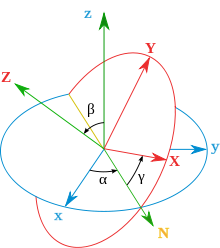
Diagram showing Euler frame in green
The components of the spin angular velocity pseudovector were first calculated by Leonhard Euler using his Euler angles and the use of an intermediate frame:
- One axis of the reference frame (the precession axis)
- The line of nodes of the moving frame with respect to the reference frame (nutation axis)
- One axis of the moving frame (the intrinsic rotation axis)
Euler proved that the projections of the angular velocity pseudovector on each of these three axes is the derivative of its associated angle (which is equivalent to decomposing the instantaneous rotation into three instantaneous Euler rotations). Therefore:[5]

This basis is not orthonormal and it is difficult to use, but now the velocity vector can be changed to the fixed frame or to the moving frame with just a change of bases. For example, changing to the mobile frame:

where  are unit vectors for the frame fixed in the moving body. This example has been made using the Z-X-Z convention for Euler angles.[citation needed]
Tensor [edit]
The angular velocity vector  defined above may be equivalently expressed as an angular velocity tensor, the matrix (or linear mapping) W = W(t) defined by:

This is an infinitesimal rotation matrix. The linear mapping W acts as  :
:

Calculation from the orientation matrix[edit]
A vector undergoing uniform circular motion around a fixed axis satisfies:

Given the orientation matrix A(t) of a frame, whose columns are the moving orthonormal coordinate vectors , we can obtain its angular velocity tensor W(t) as follows. Angular velocity must be the same for the three vectors  , so arranging the three vector equations into columns of a matrix, we have:

(This holds even if A(t) does not rotate uniformly.) Therefore the angular velocity tensor is:

since the inverse of the orthogonal matrix  is its transpose
  .
.
Properties[edit]
In general, the angular velocity in an n-dimensional space is the time derivative of the angular displacement tensor, which is a second rank skew-symmetric tensor.
This tensor W will have n(n−1)/2 independent components, which is the dimension of the Lie algebra of the Lie group of rotations of an n-dimensional inner product space.[6]
Duality with respect to the velocity vector[edit]
In three dimensions, angular velocity can be represented by a pseudovector because second rank tensors are dual to pseudovectors in three dimensions. Since the angular velocity tensor W = W(t) is a skew-symmetric matrix:

its Hodge dual is a vector, which is precisely the previous angular velocity vector ![boldsymbolomega=[omega_x,omega_y,omega_z]](https://wikimedia.org/api/rest_v1/media/math/render/svg/c8f418d52c41570663e22f7b19a8d3a427b69cab) .
.
Exponential of W[edit]
If we know an initial frame A(0) and we are given a constant angular velocity tensor W, we can obtain A(t) for any given t. Recall the matrix differential equation:
This equation can be integrated to give:

which shows a connection with the Lie group of rotations.
W is skew-symmetric[edit]
We prove that angular velocity tensor is skew symmetric, i.e.  satisfies
  .
.
A rotation matrix A is orthogonal, inverse to its transpose, so we have  . For
. For  a frame matrix, taking the time derivative of the equation gives:

Applying the formula  ,
,

Thus, W is the negative of its transpose, which implies it is skew symmetric.
Coordinate-free description[edit]
At any instant , the angular velocity tensor represents a linear map between the position vector  and the velocity vectors
  of a point on a rigid body rotating around the origin:

The relation between this linear map and the angular velocity pseudovector is the following.
Because W is the derivative of an orthogonal transformation, the bilinear form

is skew-symmetric. Thus we can apply the fact of exterior algebra that there is a unique linear form  on
on  that
that

where  is the exterior product of and
  .
.
Taking the sharp L♯ of L we get

Introducing  , as the Hodge dual of L♯, and applying the definition of the Hodge dual twice supposing that the preferred unit 3-vector is

where

by definition.
Because is an arbitrary vector, from nondegeneracy of scalar product follows

Angular velocity as a vector field[edit]
Since the spin angular velocity tensor of a rigid body (in its rest frame) is a linear transformation that maps positions to velocities (within the rigid body), it can be regarded as a constant vector field. In particular, the spin angular velocity is a Killing vector field belonging to an element of the Lie algebra SO(3) of the 3-dimensional rotation group SO(3).
Also, it can be shown that the spin angular velocity vector field is exactly half of the curl of the linear velocity vector field v(r) of the rigid body. In symbols,

Rigid body considerations[edit]
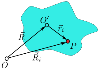
Position of point P located in the rigid body (shown in blue). Ri is the position with respect to the lab frame, centered at O and ri is the position with respect to the rigid body frame, centered at O′. The origin of the rigid body frame is at vector position R from the lab frame.
The same equations for the angular speed can be obtained reasoning over a rotating rigid body. Here is not assumed that the rigid body rotates around the origin. Instead, it can be supposed rotating around an arbitrary point that is moving with a linear velocity V(t) in each instant.
To obtain the equations, it is convenient to imagine a rigid body attached to the frames and consider a coordinate system that is fixed with respect to the rigid body. Then we will study the coordinate transformations between this coordinate and the fixed «laboratory» system.
As shown in the figure on the right, the lab system’s origin is at point O, the rigid body system origin is at O′ and the vector from O to O′ is R. A particle (i) in the rigid body is located at point P and the vector position of this particle is Ri in the lab frame, and at position ri in the body frame. It is seen that the position of the particle can be written:

The defining characteristic of a rigid body is that the distance between any two points in a rigid body is unchanging in time. This means that the length of the vector  is unchanging. By Euler’s rotation theorem, we may replace the vector with
  where
where  is a 3×3 rotation matrix and
  is the position of the particle at some fixed point in time, say t = 0. This replacement is useful, because now it is only the rotation matrix that is changing in time and not the reference vector , as the rigid body rotates about point O′. Also, since the three columns of the rotation matrix represent the three versors of a reference frame rotating together with the rigid body, any rotation about any axis becomes now visible, while the vector would not rotate if the rotation axis were parallel to it, and hence it would only describe a rotation about an axis perpendicular to it (i.e., it would not see the component of the angular velocity pseudovector parallel to it, and would only allow the computation of the component perpendicular to it). The position of the particle is now written as:

Taking the time derivative yields the velocity of the particle:

where Vi is the velocity of the particle (in the lab frame) and V is the velocity of O′ (the origin of the rigid body frame). Since is a rotation matrix its inverse is its transpose. So we substitute  :
:


or

where  is the previous angular velocity tensor.
It can be proved that this is a skew symmetric matrix, so we can take its dual to get a 3 dimensional pseudovector that is precisely the previous angular velocity vector :
Substituting ω for W into the above velocity expression, and replacing matrix multiplication by an equivalent cross product:

It can be seen that the velocity of a point in a rigid body can be divided into two terms – the velocity of a reference point fixed in the rigid body plus the cross product term involving the orbital angular velocity of the particle with respect to the reference point. This angular velocity is what physicists call the «spin angular velocity» of the rigid body, as opposed to the orbital angular velocity of the reference point O′ about the origin O.
Consistency[edit]
We have supposed that the rigid body rotates around an arbitrary point. We should prove that the spin angular velocity previously defined is independent of the choice of origin, which means that the spin angular velocity is an intrinsic property of the spinning rigid body. (Note the marked contrast of this with the orbital angular velocity of a point particle, which certainly does depend on the choice of origin.)

Proving the independence of spin angular velocity from choice of origin
See the graph to the right: The origin of lab frame is O, while O1 and O2 are two fixed points on the rigid body, whose velocity is  and
and  respectively. Suppose the angular velocity with respect to O1 and O2 is
  and
and  respectively. Since point P and O2 have only one velocity,


The above two yields that

Since the point P (and thus  ) is arbitrary, it follows that

If the reference point is the instantaneous axis of rotation the expression of the velocity of a point in the rigid body will have just the angular velocity term. This is because the velocity of the instantaneous axis of rotation is zero. An example of the instantaneous axis of rotation is the hinge of a door. Another example is the point of contact of a purely rolling spherical (or, more generally, convex) rigid body.
See also[edit]
- Angular acceleration
- Angular frequency
- Angular momentum
- Areal velocity
- Isometry
- Orthogonal group
- Rigid body dynamics
- Vorticity
References[edit]
- ^ Cummings, Karen; Halliday, David (2007). Understanding physics. New Delhi: John Wiley & Sons Inc., authorized reprint to Wiley – India. pp. 449, 484, 485, 487. ISBN 978-81-265-0882-2.(UP1)
- ^ Hibbeler, Russell C. (2009). Engineering Mechanics. Upper Saddle River, New Jersey: Pearson Prentice Hall. pp. 314, 153. ISBN 978-0-13-607791-6.(EM1)
- ^ Taylor, Barry N. (2009). International System of Units (SI) (revised 2008 ed.). DIANE Publishing. p. 27. ISBN 978-1-4379-1558-7. Extract of page 27
- ^ Singh, Sunil K. «Angular Velocity». OpenStax. Rice University. Retrieved 21 May 2021.
- ^ K.S.HEDRIH: Leonhard Euler (1707–1783) and rigid body dynamics
- ^ Rotations and Angular Momentum on the Classical Mechanics page of the website of John Baez, especially Questions 1 and 2.
- Symon, Keith (1971). Mechanics. Addison-Wesley, Reading, MA. ISBN 978-0-201-07392-8.
- Landau, L.D.; Lifshitz, E.M. (1997). Mechanics. Butterworth-Heinemann. ISBN 978-0-7506-2896-9.
External links[edit]
- A college text-book of physics By Arthur Lalanne Kimball (Angular Velocity of a particle)
- Pickering, Steve (2009). «ω Speed of Rotation [Angular Velocity]». Sixty Symbols. Brady Haran for the University of Nottingham.
| Angular velocity | |
|---|---|
|
Common symbols |
ω |
| In SI base units | s−1 |
| Extensive? | yes |
| Intensive? | yes (for rigid body only) |
| Conserved? | no |
|
Behaviour under |
pseudovector |
|
Derivations from |
ω = dθ / dt |
| Dimension | |
In physics, angular velocity or rotational velocity (ω or Ω), also known as angular frequency vector,[1] is a pseudovector representation of how fast the angular position or orientation of an object changes with time (i.e. how quickly an object rotates or revolves relative to a point or axis). The magnitude of the pseudovector represents the angular speed, the rate at which the object rotates or revolves, and its direction is normal to the instantaneous plane of rotation or angular displacement. The orientation of angular velocity is conventionally specified by the right-hand rule.[2]
There are two types of angular velocity.
- Orbital angular velocity refers to how fast a point object revolves about a fixed origin, i.e. the time rate of change of its angular position relative to the origin.
- Spin angular velocity refers to how fast a rigid body rotates with respect to its center of rotation and is independent of the choice of origin, in contrast to orbital angular velocity.
In general, angular velocity has dimension of angle per unit time (angle replacing distance from linear velocity with time in common). The SI unit of angular velocity is radians per second,[3] with the radian being a dimensionless quantity, thus the SI units of angular velocity may be listed as s−1. Angular velocity is usually represented by the symbol omega (ω, sometimes Ω). By convention, positive angular velocity indicates counter-clockwise rotation, while negative is clockwise.
For example, a geostationary satellite completes one orbit per day above the equator, or 360 degrees per 24 hours, and has angular velocity ω = (360°)/(24 h) = 15°/h, or (2π rad)/(24 h) ≈ 0.26 rad/h. If angle is measured in radians, the linear velocity is the radius times the angular velocity, . With orbital radius 42,000 km from the earth’s center, the satellite’s speed through space is thus v = 42,000 km × 0.26/h ≈ 11,000 km/h. The angular velocity is positive since the satellite travels eastward with the Earth’s rotation (counter-clockwise from above the north pole.)
Orbital angular velocity of a point particle[edit]
Particle in two dimensions[edit]
The angular velocity of the particle at P with respect to the origin O is determined by the perpendicular component of the velocity vector v.
In the simplest case of circular motion at radius , with position given by the angular displacement from the x-axis, the orbital angular velocity is the rate of change of angle with respect to time: . If is measured in radians, the arc-length from the positive x-axis around the circle to the particle is , and the linear velocity is , so that .
In the general case of a particle moving in the plane, the orbital angular velocity is the rate at which the position vector relative to a chosen origin «sweeps out» angle. The diagram shows the position vector from the origin to a particle , with its polar coordinates . (All variables are functions of time .) The particle has linear velocity splitting as , with the radial component parallel to the radius, and the cross-radial (or tangential) component perpendicular to the radius. When there is no radial component, the particle moves around the origin in a circle; but when there is no cross-radial component, it moves in a straight line from the origin. Since radial motion leaves the angle unchanged, only the cross-radial component of linear velocity contributes to angular velocity.
The angular velocity ω is the rate of change of angular position with respect to time, which can be computed from the cross-radial velocity as:
Here the cross-radial speed is the signed magnitude of , positive for counter-clockwise motion, negative for clockwise. Taking polar coordinates for the linear velocity gives magnitude (linear speed) and angle relative to the radius vector; in these terms, , so that
These formulas may be derived doing , being a function of the distance to the origin with respect to time, and a function of the angle between the vector and the x axis. Then . Which is equal to . (See Unit vector in cylindrical coordinates). Knowing , we conclude that the radial component of the velocity is given by , because is a radial unit vector; and the perpendicular component is given by because is a perpendicular unit vector.
In two dimensions, angular velocity is a number with plus or minus sign indicating orientation, but not pointing in a direction. The sign is conventionally taken to be positive if the radius vector turns counter-clockwise, and negative if clockwise. Angular velocity then may be termed a pseudoscalar, a numerical quantity which changes sign under a parity inversion, such as inverting one axis or switching the two axes.
Particle in three dimensions[edit]
The orbital angular velocity vector encodes the time rate of change of angular position, as well as the instantaneous plane of angular displacement. In this case (counter-clockwise circular motion) the vector points up.
In three-dimensional space, we again have the position vector r of a moving particle. Here, orbital angular velocity is a pseudovector whose magnitude is the rate at which r sweeps out angle, and whose direction is perpendicular to the instantaneous plane in which r sweeps out angle (i.e. the plane spanned by r and v). However, as there are two directions perpendicular to any plane, an additional condition is necessary to uniquely specify the direction of the angular velocity; conventionally, the right-hand rule is used.
Let the pseudovector be the unit vector perpendicular to the plane spanned by r and v, so that the right-hand rule is satisfied (i.e. the instantaneous direction of angular displacement is counter-clockwise looking from the top of ). Taking polar coordinates in this plane, as in the two-dimensional case above, one may define the orbital angular velocity vector as:
where θ is the angle between r and v. In terms of the cross product, this is:
- [4]
From the above equation, one can recover the tangential velocity as:
Spin angular velocity of a rigid body or reference frame[edit]
Given a rotating frame of three unit coordinate vectors, all the three must have the same angular speed at each instant. In such a frame, each vector may be considered as a moving particle with constant scalar radius.
The rotating frame appears in the context of rigid bodies, and special tools have been developed for it: the spin angular velocity may be described as a vector or equivalently as a tensor.
Consistent with the general definition, the spin angular velocity of a frame is defined as the orbital angular velocity of any of the three vectors (same for all) with respect to its own center of rotation. The addition of angular velocity vectors for frames is also defined by the usual vector addition (composition of linear movements), and can be useful to decompose the rotation as in a gimbal. All components of the vector can be calculated as derivatives of the parameters defining the moving frames (Euler angles or rotation matrices). As in the general case, addition is commutative: .
By Euler’s rotation theorem, any rotating frame possesses an instantaneous axis of rotation, which is the direction of the angular velocity vector, and the magnitude of the angular velocity is consistent with the two-dimensional case.
If we choose a reference point fixed in the rigid body, the velocity of any point in the body is given by
Components from the basis vectors of a body-fixed frame[edit]
Consider a rigid body rotating about a fixed point O. Construct a reference frame in the body consisting of an orthonormal set of vectors fixed to the body and with their common origin at O. The spin angular velocity vector of both frame and body about O is then
where is the time rate of change of the frame vector due to the rotation.
Note that this formula is incompatible with the expression for orbital angular velocity
as that formula defines angular velocity for a single point about O, while the formula in this section applies to a frame or rigid body. In the case of a rigid body a single has to account for the motion of all particles in the body.
Components from Euler angles[edit]
Diagram showing Euler frame in green
The components of the spin angular velocity pseudovector were first calculated by Leonhard Euler using his Euler angles and the use of an intermediate frame:
- One axis of the reference frame (the precession axis)
- The line of nodes of the moving frame with respect to the reference frame (nutation axis)
- One axis of the moving frame (the intrinsic rotation axis)
Euler proved that the projections of the angular velocity pseudovector on each of these three axes is the derivative of its associated angle (which is equivalent to decomposing the instantaneous rotation into three instantaneous Euler rotations). Therefore:[5]
This basis is not orthonormal and it is difficult to use, but now the velocity vector can be changed to the fixed frame or to the moving frame with just a change of bases. For example, changing to the mobile frame:
where are unit vectors for the frame fixed in the moving body. This example has been made using the Z-X-Z convention for Euler angles.[citation needed]
Tensor [edit]
The angular velocity vector defined above may be equivalently expressed as an angular velocity tensor, the matrix (or linear mapping) W = W(t) defined by:
This is an infinitesimal rotation matrix. The linear mapping W acts as :
Calculation from the orientation matrix[edit]
A vector undergoing uniform circular motion around a fixed axis satisfies:
Given the orientation matrix A(t) of a frame, whose columns are the moving orthonormal coordinate vectors , we can obtain its angular velocity tensor W(t) as follows. Angular velocity must be the same for the three vectors , so arranging the three vector equations into columns of a matrix, we have:
(This holds even if A(t) does not rotate uniformly.) Therefore the angular velocity tensor is:
since the inverse of the orthogonal matrix is its transpose .
Properties[edit]
In general, the angular velocity in an n-dimensional space is the time derivative of the angular displacement tensor, which is a second rank skew-symmetric tensor.
This tensor W will have n(n−1)/2 independent components, which is the dimension of the Lie algebra of the Lie group of rotations of an n-dimensional inner product space.[6]
Duality with respect to the velocity vector[edit]
In three dimensions, angular velocity can be represented by a pseudovector because second rank tensors are dual to pseudovectors in three dimensions. Since the angular velocity tensor W = W(t) is a skew-symmetric matrix:
its Hodge dual is a vector, which is precisely the previous angular velocity vector .
Exponential of W[edit]
If we know an initial frame A(0) and we are given a constant angular velocity tensor W, we can obtain A(t) for any given t. Recall the matrix differential equation:
This equation can be integrated to give:
which shows a connection with the Lie group of rotations.
W is skew-symmetric[edit]
We prove that angular velocity tensor is skew symmetric, i.e. satisfies .
A rotation matrix A is orthogonal, inverse to its transpose, so we have . For a frame matrix, taking the time derivative of the equation gives:
Applying the formula ,
Thus, W is the negative of its transpose, which implies it is skew symmetric.
Coordinate-free description[edit]
At any instant , the angular velocity tensor represents a linear map between the position vector and the velocity vectors of a point on a rigid body rotating around the origin:
The relation between this linear map and the angular velocity pseudovector is the following.
Because W is the derivative of an orthogonal transformation, the bilinear form
is skew-symmetric. Thus we can apply the fact of exterior algebra that there is a unique linear form on that
where is the exterior product of and .
Taking the sharp L♯ of L we get
Introducing , as the Hodge dual of L♯, and applying the definition of the Hodge dual twice supposing that the preferred unit 3-vector is
where
by definition.
Because is an arbitrary vector, from nondegeneracy of scalar product follows
Angular velocity as a vector field[edit]
Since the spin angular velocity tensor of a rigid body (in its rest frame) is a linear transformation that maps positions to velocities (within the rigid body), it can be regarded as a constant vector field. In particular, the spin angular velocity is a Killing vector field belonging to an element of the Lie algebra SO(3) of the 3-dimensional rotation group SO(3).
Also, it can be shown that the spin angular velocity vector field is exactly half of the curl of the linear velocity vector field v(r) of the rigid body. In symbols,
Rigid body considerations[edit]
Position of point P located in the rigid body (shown in blue). Ri is the position with respect to the lab frame, centered at O and ri is the position with respect to the rigid body frame, centered at O′. The origin of the rigid body frame is at vector position R from the lab frame.
The same equations for the angular speed can be obtained reasoning over a rotating rigid body. Here is not assumed that the rigid body rotates around the origin. Instead, it can be supposed rotating around an arbitrary point that is moving with a linear velocity V(t) in each instant.
To obtain the equations, it is convenient to imagine a rigid body attached to the frames and consider a coordinate system that is fixed with respect to the rigid body. Then we will study the coordinate transformations between this coordinate and the fixed «laboratory» system.
As shown in the figure on the right, the lab system’s origin is at point O, the rigid body system origin is at O′ and the vector from O to O′ is R. A particle (i) in the rigid body is located at point P and the vector position of this particle is Ri in the lab frame, and at position ri in the body frame. It is seen that the position of the particle can be written:
The defining characteristic of a rigid body is that the distance between any two points in a rigid body is unchanging in time. This means that the length of the vector is unchanging. By Euler’s rotation theorem, we may replace the vector with where is a 3×3 rotation matrix and is the position of the particle at some fixed point in time, say t = 0. This replacement is useful, because now it is only the rotation matrix that is changing in time and not the reference vector , as the rigid body rotates about point O′. Also, since the three columns of the rotation matrix represent the three versors of a reference frame rotating together with the rigid body, any rotation about any axis becomes now visible, while the vector would not rotate if the rotation axis were parallel to it, and hence it would only describe a rotation about an axis perpendicular to it (i.e., it would not see the component of the angular velocity pseudovector parallel to it, and would only allow the computation of the component perpendicular to it). The position of the particle is now written as:
Taking the time derivative yields the velocity of the particle:
where Vi is the velocity of the particle (in the lab frame) and V is the velocity of O′ (the origin of the rigid body frame). Since is a rotation matrix its inverse is its transpose. So we substitute :
or
where is the previous angular velocity tensor.
It can be proved that this is a skew symmetric matrix, so we can take its dual to get a 3 dimensional pseudovector that is precisely the previous angular velocity vector :
Substituting ω for W into the above velocity expression, and replacing matrix multiplication by an equivalent cross product:
It can be seen that the velocity of a point in a rigid body can be divided into two terms – the velocity of a reference point fixed in the rigid body plus the cross product term involving the orbital angular velocity of the particle with respect to the reference point. This angular velocity is what physicists call the «spin angular velocity» of the rigid body, as opposed to the orbital angular velocity of the reference point O′ about the origin O.
Consistency[edit]
We have supposed that the rigid body rotates around an arbitrary point. We should prove that the spin angular velocity previously defined is independent of the choice of origin, which means that the spin angular velocity is an intrinsic property of the spinning rigid body. (Note the marked contrast of this with the orbital angular velocity of a point particle, which certainly does depend on the choice of origin.)
Proving the independence of spin angular velocity from choice of origin
See the graph to the right: The origin of lab frame is O, while O1 and O2 are two fixed points on the rigid body, whose velocity is and respectively. Suppose the angular velocity with respect to O1 and O2 is and respectively. Since point P and O2 have only one velocity,
The above two yields that
Since the point P (and thus ) is arbitrary, it follows that
If the reference point is the instantaneous axis of rotation the expression of the velocity of a point in the rigid body will have just the angular velocity term. This is because the velocity of the instantaneous axis of rotation is zero. An example of the instantaneous axis of rotation is the hinge of a door. Another example is the point of contact of a purely rolling spherical (or, more generally, convex) rigid body.
See also[edit]
- Angular acceleration
- Angular frequency
- Angular momentum
- Areal velocity
- Isometry
- Orthogonal group
- Rigid body dynamics
- Vorticity
References[edit]
- ^ Cummings, Karen; Halliday, David (2007). Understanding physics. New Delhi: John Wiley & Sons Inc., authorized reprint to Wiley – India. pp. 449, 484, 485, 487. ISBN 978-81-265-0882-2.(UP1)
- ^ Hibbeler, Russell C. (2009). Engineering Mechanics. Upper Saddle River, New Jersey: Pearson Prentice Hall. pp. 314, 153. ISBN 978-0-13-607791-6.(EM1)
- ^ Taylor, Barry N. (2009). International System of Units (SI) (revised 2008 ed.). DIANE Publishing. p. 27. ISBN 978-1-4379-1558-7. Extract of page 27
- ^ Singh, Sunil K. «Angular Velocity». OpenStax. Rice University. Retrieved 21 May 2021.
- ^ K.S.HEDRIH: Leonhard Euler (1707–1783) and rigid body dynamics
- ^ Rotations and Angular Momentum on the Classical Mechanics page of the website of John Baez, especially Questions 1 and 2.
- Symon, Keith (1971). Mechanics. Addison-Wesley, Reading, MA. ISBN 978-0-201-07392-8.
- Landau, L.D.; Lifshitz, E.M. (1997). Mechanics. Butterworth-Heinemann. ISBN 978-0-7506-2896-9.
External links[edit]
- A college text-book of physics By Arthur Lalanne Kimball (Angular Velocity of a particle)
- Pickering, Steve (2009). «ω Speed of Rotation [Angular Velocity]». Sixty Symbols. Brady Haran for the University of Nottingham.
Рассмотрим понятия угловой скорости и углового ускорения при вращении твердого тела в теории и на примерах решения задач.
Угловая скорость
Угловой скоростью называют скорость вращения тела, определяющуюся приращением угла поворота тела за некоторый промежуток (единицу) времени.
Обозначение угловой скорости: ω (омега).
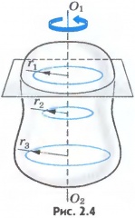
Рассмотрим некоторое твердое тело, вращающееся относительно неподвижной оси.
С этим телом свяжем воображаемую плоскость П, которая совершает вращение вместе с заданным телом.
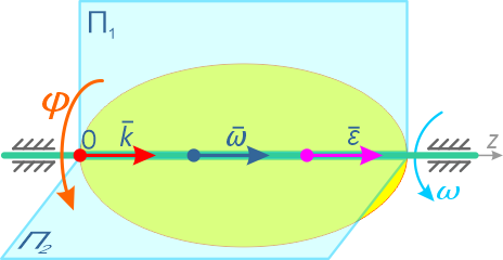
Вращательное движение определяется двугранным углом φ между двумя плоскостями, проходящими через ось вращения. Изменение этого угла с течением времени есть закон вращательного движения:
Положительным считается угол, откладываемый против хода часовой стрелки, если смотреть навстречу выбранному направлению оси вращения Oz. Угол измеряется в радианах.
Быстрота изменения угла φ (перемещения плоскости П из положения П1 в положение П2) – это и есть угловая скорость:
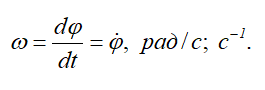
Приняв вектор k как единичный орт положительного направления оси, получим:
Вектор угловой скорости – скользящий вектор: он может быть приложен к любой точке оси вращения и всегда направлен вдоль оси, при положительном значении угловой скорости направления ω и k совпадают, при отрицательном – противоположны.
Формулы угловой скорости
Формула для расчета угловой скорости в зависимости от заданных параметров вращения может иметь вид:
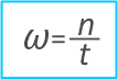
- если известно количество оборотов n за единицу времени t:

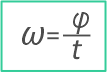
- если задан угол поворота φ за единицу времени:
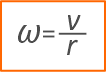
- если известна окружная скорость точки тела v и расстояние от оси вращения до этой точки r:

Размерности угловой скорости:
- Количество оборотов за единицу времени [об/мин], [c-1].
- Угол поворота за единицу времени [рад/с].
Определение угловой скорости
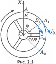
Пример: Диск вращается относительно своего центра.
Известна скорость v некоторой точки A, расположенной на расстоянии r от центра вращения диска.
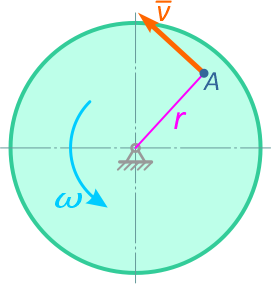
Определить величину и направление угловой скорости диска ω, если v = 5 м/с, r = 70 см.
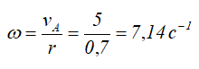
Таким образом, угловая скорость диска составляет 7,14 оборотов в секунду. Направление угловой скорости можно определить по направлению скоростей её точек.
Вектор скорости точки A стремится повернуть диск относительно центра вращения против хода часовой стрелки, следовательно, направление угловой скорости вращения диска имеет такое же направление.
Другие примеры решения задач >
Угловое ускорение
Угловое ускорение характеризует величину изменения угловой скорости при вращении твердого тела:
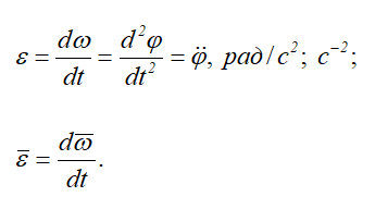
Обозначение: ε (Эпсилон)
Единицы измерения углового ускорения: [рад/с2], [с-2]
Вектор углового ускорения так же направлен по оси вращения. При ускоренном вращении их направления совпадают, при замедленном — противоположны.
Другими словами, при положительном ускорении угловая скорость нарастает (вращение ускоряется), а при отрицательном — уменьшается (вращение замедляется).
Для некоторых частных случаев вращательного движения твердого тела могут быть использованы формулы:
Расчет углового ускорения
Пример: По заданному значению касательной составляющей полного ускорения aτ точки B, расположенной на расстоянии r от центра вращения колеса.
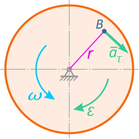
Требуется определить величину и направление углового ускорения колеса ε, если aτ = 10 м/с2, r = 50 см.
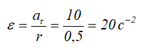
Угловое ускорение колеса в заданный момент времени составляет 20 оборотов за секунду в квадрате. Направление углового ускорения определяется по направлению тангенциального ускорения точки.
Здесь, угловое ускорение направлено противоположно направлению угловой скорости вращения колеса. Это означает, что вращение колеса замедляется.
В технике угловая скорость часто задается в оборотах в минуту n [об/мин]. Один оборот – это 2π радиан:
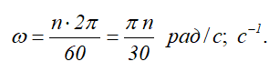
Например, тело совершающее 1,5 оборота за одну секунду имеет угловую скорость
ω = 1,5 с-1 = 9,42 рад/с.
Смотрите также:
- Примеры расчета угловой скорости и ускорения
- Скорости и ускорения точек вращающегося тела
Что такое угловая скорость
Угловая скорость (обозначается как (omega)) — векторная величина, характеризующая скорость и направление изменения угла поворота со временем.
Модуль угловой скорости для вращательного движения совпадает с мгновенной угловой частотой вращения, а направление перпендикулярно плоскости вращения и связано с направлением вращения правилом правого винта.
Единица измерения
В Международной системе единиц (СИ) принятой единицей измерения угловой скорости является радиан в секунду (рад/с)
Осторожно! Если преподаватель обнаружит плагиат в работе, не избежать крупных проблем (вплоть до отчисления). Если нет возможности написать самому, закажите тут.
Формула угловой скорости
Вектор угловой скорости определяется отношением угла поворота ((varphi)) к интервалу времени ((mathcal t)), за которое произошел поворот:
(omega=frac{trianglevarphi}{trianglemathcal t})
Зависимость угловой скорости от времени
Зависимость (varphi ) от (mathcal t) наглядно показана на графике:
Угол, на который повернулось тело, характеризуется площадью под кривой.
Угловая скорость вращения, формула
Через частоту
(omega=2pimathcal n)
(mathcal n) — частота вращения ((1/с))
(pi) — число Пи ((approx 3,14))
(mathcal n=frac1T)
(T )— период вращения (время, за которое тело совершает один оборот)
Через радиус
(omega=frac vR)
(v) — линейная скорость(м/с)
(R) — радиус окружности (м)
Как определить направление угловой скорости
Направление скорости в физике можно определять двумя способами:
- Правило буравчика. Буравчик имеет правую резьбу (вращательное движение вправо при закручивании). Если вращать буравчик в направлении вращения тела, он будет завинчиваться (или вывинчиваться) в ту сторону, куда направлена угловая скорость.
- Правило правой руки. Представим, что взяли тело в правую руку. Следует направлять и вращать его туда, куда указывают четыре пальца. Отведенный в сторону большой палец покажет направление угловой скорости при этом вращении.
Связь линейной и угловой скорости
Линейная скорость ((v)) тела, расположенного на расстоянии (R) от оси вращения, прямо пропорциональна угловой скорости.
(v=Romega)
(R) — радиус окружности (м)
Чему равна мгновенная угловая скорость
Мгновенную угловую скорость нужно находить как предел, к которому стремится средняя угловая скорость при (trianglemathcal trightarrow0) :
(omega=lim_{trianglerightarrow0}frac{trianglevarphi}{trianglemathcal t})
Измеряется в рад/с
Содержание:
- Определение и формула угловой скорости
- Равномерное вращение
- Формула, связывающая линейную и угловую скорости
- Единицы измерения угловой скорости
- Примеры решения задач
Определение и формула угловой скорости
Определение
Круговым движением точки вокруг некоторой оси называют движение, при котором траекторией точки является окружность
с центром, который лежит на оси вращения, при этом плоскость окружности перпендикулярна этой оси.
Вращением тела вокруг оси называют движение, при котором все точки тела совершают круговые движения около этой оси.
Перемещение при вращении характеризуют при помощи угла поворота
$(varphi)$ . Часто используют вектор элементарного поворота
$bar{dvarphi}$ , который равен по величине элементарному углу поворота тела
$(d varphi)$ за маленький отрезок времени dt и направлен по мгновенной оси вращения в сторону,
откуда этот поворот виден реализующимся против часовой стрелки. Надо отметить, что только элементарные угловые перемещения являются векторами.
Углы вращения на конечные величины векторами не являются.
Определение
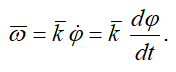
Угловой скоростью называют скорость изменения угла поворота и обозначают ее обычно буквой
$omega$ . Математически определение угловой скорости записывают так:
$$bar{omega}=frac{d bar{varphi}}{d t}=dot{bar{varphi}}(1)$$
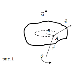
Угловая скорость — векторная величина (это аксиальный вектор). Она имеет направление вдоль мгновенной оси вращения совпадающее
с направлением поступательного правого винта, если его вращать в сторону вращения тела (рис.1).
Вектор угловой скорости может претерпевать изменения как за счет изменения скорости вращения тела вокруг оси (изменение модуля угловой скорости),
так и за счет поворота оси вращения в пространстве ($bar{omega}$ при этом изменяет направление).
Равномерное вращение
Если тело за равные промежутки времени поворачивается на один и тот же угол,
то такое вращение называют равномерным. При этом модуль угловой скорости находят как:
$$omega=frac{varphi}{t}(2)$$
где $(varphi)$ – угол поворота, t – время, за которое этот поворот совершён.
Равномерное вращение часто характеризуют при помощи периода обращения (T), который является временем, за которое тело производит один оборот
($Delta varphi=2 pi$). Угловая скорость связана с периодом обращения как:
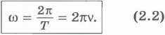
$$omega=frac{2 pi}{T}(3)$$
С числом оборотов в единицу времени ($nu) угловая скорость связана формулой:
$$omega=2 pi nu(4)$$
Понятия периода обращения и числа оборотов в единицу времени иногда используют и для описания неравномерного вращения,
но понимают при этом под мгновенным значением T, время за которое тело делало бы один оборот, если бы оно вращалось равномерно
с данной мгновенной величиной скорости.
Формула, связывающая линейную и угловую скорости
Линейная скорость $bar{v}$ точки А (рис.1), которая расположена
на расстоянии R от оси вращения связана с вектором угловой скорости следующим векторным произведением:
$$bar{v}=[bar{omega} bar{R}](5)$$
где $bar{R}$ – перпендикулярная к оси вращения компонента радиус-вектора точки
$A (bar{r})$ (рис.1). Вектор
$bar{r}$ проводят от точки, находящейся на оси вращения к рассматриваемой точке.
Единицы измерения угловой скорости
Основной единицей измерения угловой скорости в системе СИ является: [$omega$]=рад/с
В СГС: [$omega$]=рад/с
Примеры решения задач
Пример
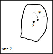
Задание. Движение тела с неподвижной осью задано уравнением
$varphi=2 t-4 t^{3}$,
$(varphi)$ в рад, t в сек.
Начало вращения при t=0 c. Положительным считают углы указанные направлением стрелки (рис.2). В каком направлении (
относительно часовой стрелки поворачивается тело) в момент времени t=0,5 c.
Решение. Для нахождения модуля угловой скорости применим формулу:
$$omega=frac{d varphi}{d t}(1.1)$$
Используем заданную в условии задачи функцию
$varphi(t)$, возьмем производную от нее по времени, получим функцию
$omega(t)$:
$$omega(t)=2-8 t^{2}(1.2)$$
Вычислим, чему будет равна угловая скорость в заданный момент времени (при t=0,5 c):
$$omega(t)=2-8(0,5)^{2}=0left(frac{r a d}{c}right)$$
Ответ. В заданный момент времени тело имеет угловую скорость равную нулю, следовательно, она останавливается.

236
проверенных автора готовы помочь в написании работы любой сложности
Мы помогли уже 4 396 ученикам и студентам сдать работы от решения задач до дипломных на отлично! Узнай стоимость своей работы за 15 минут!
Пример
Задание. Скорости вращения тела заданы системой уравнений:
$$left{begin{array}{c}bar{omega}_{1}=t^{2 bar{i}} \ bar{omega}_{2}=2 t^{2} bar{j}end{array}right.$$
где $bar{i}$ и
$bar{j}$ – единичные ортогональные векторы. На какой угол $(varphi)$ поворачивается тело за время равное 3 с?
Решение. Определим, какова функция, которая связывает модуль скорости вращения тела и время (t)
($omega(t)$). Так как вектора
$bar{i}$ и
$bar{j}$ перпендикулярны друг другу, значит:
$$omega=sqrt{omega_{1}^{2}+omega_{2}^{2}}=sqrt{left(t^{2}right)^{2}+left(2 t^{2}right)^{2}}=t^{2} sqrt{5}(2.2)$$
Модуль угловой скорости связан с углом поворота как:
$$omega=frac{d varphi}{d t}(2.3)$$
Следовательно, угол поворота найдем как:
$$varphi=int_{t_{1}}^{t_{2}} omega d t=int_{0}^{3} t^{2} sqrt{5} d t=left.sqrt{5} frac{t^{3}}{3}right|_{0} ^{3} approx 20(mathrm{rad})$$
Ответ. $varphi = 20$ рад.
Читать дальше: Формула удельного веса.
| Угловая скорость | |
 |
|
| Размерность |
T −1 |
|---|---|
| Единицы измерения | |
| СИ |
рад/с |
| СГС |
рад/с |
| Другие единицы |
градус/с, оборот/с, оборот/мин |


![]()
Угловая скорость (синяя стрелка) в полторы единицы по часовой стрелке

![]()
Угловая скорость (синяя стрелка) в одну единицу против часовой стрелки
Углова́я ско́рость — векторная физическая величина, характеризующая скорость вращения тела. Вектор угловой скорости по величине равен углу поворота тела в единицу времени:
- ,
 ,
,а направлен по оси вращения согласно правилу буравчика, то есть, в ту сторону, в которую ввинчивался бы буравчик с правой резьбой, если бы вращался в ту же сторону.
Единица измерения угловой скорости, принятая в системах СИ и СГС — радианы в секунду. (Примечание: радиан, как и любые единицы измерения угла, — физически безразмерен, поэтому физическая размерность угловой скорости — просто [1/секунда]). В технике также используются обороты в секунду, намного реже — градусы в секунду, грады в секунду. Пожалуй, чаще всего в технике используют обороты в минуту — это идёт с тех времён, когда частоту вращения тихоходных паровых машин определяли просто «вручную», подсчитывая число оборотов за единицу времени.
Вектор (мгновенной) скорости любой точки (абсолютно) твердого тела, вращающегося с угловой скоростью  , определяется формулой:
![vec v = [ vec omega, vec r ],](https://dic.academic.ru/dic.nsf/ruwiki/3a29410b481fbe1233e57e7d11022027.png)
где  — радиус-вектор к данной точке из начала координат, расположенного на оси вращения тела, а квадратными скобками обозначено векторное произведение. Линейную скорость (совпадающую с модулем вектора скорости) точки на определенном расстоянии (радиусе)
  от оси вращения можно считать так:
  Если вместо радианов применять другие единицы углов, то в двух последних формулах появится множитель, не равный единице.
- В случае плоского вращения, то есть когда все векторы скоростей точек тела лежат (всегда) в одной плоскости («плоскости вращения»), угловая скорость тела всегда перпендикулярна этой плоскости, и по сути — если плоскость вращения заведомо известна — может быть заменена скаляром — проекцией на ось, ортогональную плоскости вращения. В этом случае кинематика вращения сильно упрощается, однако в общем случае угловая скорость может менять со временем направление в трехмерном пространстве, и такая упрощенная картина не работает.
- Производная угловой скорости по времени есть угловое ускорение.
- Движение с постоянным вектором угловой скорости называется равномерным вращательным движением (в этом случае угловое ускорение равно нулю).
- Угловая скорость (рассматриваемая как свободный вектор) одинакова во всех инерциальных системах отсчета, однако в разных инерциальных системах отсчета может различаться ось или центр вращения одного и того же конкретного тела в один и тот же момент времени (то есть будет различной «точка приложения» угловой скорости).
- В случае движения одной единственной точки в трехмерном пространстве можно написать выражение для угловой скорости этой точки относительно выбранного начала координат:
- , где — радиус-вектор точки (из начала координат), — скорость этой точки. — векторное произведение, — скалярное произведение векторов. Однако эта формула не определяет угловую скорость однозначно (в случае единственной точки можно подобрать и другие векторы , подходящие по определению, по другому — произвольно — выбрав направление оси вращения), а для общего случая (когда тело включает более одной материальной точки) — эта формула не верна для угловой скорости всего тела (так как дает разные для каждой точки, а при вращении абсолютно твёрдого тела по определению угловая скорость его вращения — единственный вектор). При всём при этом, в двумерном случае (случае плоского вращения) эта формула вполне достаточна, однозначна и корректна, так как в этом частном случае направление оси вращения заведомо однозначно определено.
 , где
, где  — скорость этой точки.
  — векторное произведение,
  — скалярное произведение векторов. Однако эта формула не определяет угловую скорость однозначно (в случае единственной точки можно подобрать и другие векторы
 - В случае равномерного вращательного движения (то есть движения с постоянным вектором угловой скорости) декартовы координаты точек вращающегося так тела совершают гармонические колебания с угловой (циклической) частотой, равной модулю вектора угловой скорости.
Связь с конечным поворотом в пространстве
- .
 .
.- .
 .
.- .
 .
.См. также
- Угловая частота
- Угловое ускорение
- Момент импульса
Литература
- Лурье А. И. Аналитическая механика\ А. И. Лурье. — М.: ГИФМЛ, 1961. — С. 100-136
Рассмотрим
твердое тело, которое вращается
вокруг неподвижной оси. Тогда отдельные
точки этого тела будут описывать
окружности разных радиусов, центры
которых лежат на оси вращения. Пусть
некоторая точка движется по окружности
радиуса R
(рис.6).
Ее положение через промежуток времени
t
зададим
углом .
Элементарные (бесконечно малые) углы
поворота рассматривают как векторы.
Модуль вектора d
равен
углу поворота, а его направление совпадает
с направлением поступательного
движения острия винта, головка которого
вращается в направлении движения
точки по окружности, т. е. подчиняется
правилу
правого, винта (рис.6).
Векторы, направления которых связываются
с направлением вращения, называются
псевдовекторами
или
аксиальными
векторами. Эти
векторы не имеют определенных точек
приложения: они могут откладываться
из любой точки оси вращения.
Угловой
скоростью называется
векторная величина, равная первой
производной угла поворота тела по
времени:

Вектор
«в направлен вдоль оси вращения по
правилу правого винта, т. е. так же, как
и вектор d
(рис. 7). Размерность угловой скорости
dim=T-1,
a .
ее единица — радиан в секунду (рад/с).
Линейная скорость
точки (см. рис. 6)

В векторном виде
формулу для линейной скорости можно
написать как векторное произведение:
![]()
При
этом модуль векторного произведения,
по определению, равен
![]()
,
а
направление совпадает с
направлением
поступательного движения правого винта
при его вращении от
к R.
Если
=const,
то
вращение равномерное и его можно
характеризовать периодом
вращения Т
—
временем, за которое точка совершает
один полный оборот, т. е. поворачивается
на угол 2.
Так как промежутку времени t=T
соответствует =2,
то =
2/Т,
откуда
![]()
Число
полных оборотов, совершаемых телом при
равномерном его движении по окружности,
в единицу времени называется частотой
вращения:

Угловым
ускорением называется
векторная величина, равная первой
производной угловой скорости по
времени:

При вращении тела
вокруг неподвижной оси вектор углового
ускорения направлен вдоль оси вращения
в сторону вектора элементарного
приращения угловой скорости. При
ускоренном движении вектор
13
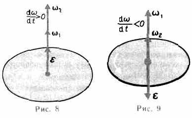
сонаправлен
вектору
(рис.8),
при замедленном.— противонаправлен
ему (рис. 9).
Тангенциальная
составляющая ускорения

Нормальная
составляющая ускорения
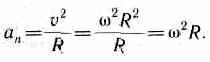
Таким
образом, связь между линейными (длина
пути s,
пройденного
точкой по дуге окружности радиуса R,
линейная
скорость v,
тангенциальное
ускорение а,
нормальное ускорение аn)
и угловыми величинами (угол поворота
,
угловая скорость (о, угловое ускорение
)
выражается следующими формулами:
![]()
В
случае равнопеременного движения точки
по окружности (=const)
![]()
где
0
— начальная угловая скорость.
Контрольные
вопросы
• Что
называется материальной точкой? Почему
в механике вводят такую модель?
• Что
такое система отсчета?
• Что
такое вектор перемещения? Всегда ли
модуль вектора перемещения равен отрезку
пути,
пройденному точкой?
• Какое
движение называется поступательным?
вращательным?
• Дать
определения векторов средней скорости
и среднего ускорения, мгновенной
скорости
и мгновенного
ускорения. Каковы их направления?
• Что
характеризует тангенциальная
составляющая ускорения? нормальная
составляющая
ускорения? Каковы
их модули?
• Возможны
ли движения, при которых отсутствует
нормальное ускорение? тангенциальное
ускорение? Приведите
примеры.
• Что
называется угловой скоростью? угловым
ускорением? Как определяются их
направления?
• Какова
связь между линейными и угловыми
величинами?
Задачи
1.1.
Зависимость
пройденного телом пути от времени
задается уравнением s
= A+Вt+Сt2+Dt3
(С
= 0,1 м/с2,
D
= 0,03 м/с3).
Определить: 1) через какое время после
начала движения ускорение а тела будет
равно 2 м/с2;
2) среднее ускорение <а>
тела за этот промежуток времени. [ 1) 10
с; 2) 1,1 м/с2]
1.2.
Пренебрегая сопротивлением воздуха,
определить угол, под которым тело брошено
к горизонту, если максимальная высота
подъема тела равна 1/4 дальности его
полета. [45°]
1.3.
Колесо
радиуса R
=
0,1 м вращается так, что зависимость
угловой скорости от времени задается
уравнением
= 2At+5Вt4
(A=2
рад/с2
и B=1
рад/с5).
Определить полное ускорение точек обода
колеса через t=1
с после начала вращения и число оборотов,
сделанных колесом за это время. [а =
8,5 м/с2;
N
= 0,48]
14
1.4.
Нормальное ускорение точки, движущейся
по окружности радиуса r=4
м,
задается уравнением аn=А+-Bt+Ct2
(A=1
м/с2,
В=6
м/с3,
С=3
м/с4).
Определить: 1) тангенциальное ускорение
точки; 2) путь, пройденный точкой за время
t1=5
с после начала движения; 3) полное
ускорение для момента времени t2=1
с. [ 1) 6 м/с2;
2) 85 м; 3) 6,32 м/с2]
1.5.
Частота
вращения колеса при равнозамедленном
движении за t=1
мин
уменьшилась от 300 до 180 мин-1.
Определить: 1) угловое ускорение колеса;
2) число полных оборотов, сделанных
колесом за это время. [1)
0,21 рад/с2;
2) 360]
1.6.
Диск
радиусом R=10
см вращается вокруг неподвижной оси
так, что зависимость угла поворота
радиуса диска от времени задается
уравнением =A+Bt+Ct2+Dt3
(B
= l рад/с,
С=1
рад/с2,
D=l
рад/с3).
Определить для точек на ободе колеса к
концу второй секунды после начала
движения: 1) тангенциальное ускорение
а;
2) нормальное ускорение аn;
3) полное ускорение а. [ 1) 0,14 м/с2;
2) 28,9 м/с2;
3) 28,9 м/с2]
Соседние файлы в папке Трофимова
- #
- #
- #
- #
- #
- #
|
1.9.2 Угловая и линейная скорости вращения
|